Getting Started with pmforest
Kyle Barrett
Source:vignettes/getting-started.Rmd
getting-started.RmdIntroduction/Scope
pmforest is a package for producing forest plots:
graphical summaries of covariate effects or covariate-dependent
predictions in a pharmacometric model.
Given a dataset of model responses or model parameters with uncertainty at various covariate levels, the package generates plots of confidence intervals reflecting the predicted impact of the covariates. This uncertainty could come from a variety of sources, for example: simulations, bootstrapping, Bayesian posteriors.
Input data
To use the forest plot function you will have raw data coming from
something like simulations. Before plotting, the raw data must first be
summarized. To help with this, pmforest has a summarize_data()
function. The usage of this function is described in the next section,
but note that the user can write their own custom summarization
function, as long as the data it returns conforms to the format
described in the “Output Data” section of ?summarize_data.
Raw data
The raw dataset must be in long format and have the following:
- A numeric column containing the values to be summarized (passed to
valueargument ofsummarize_data()). - A character (or factor) column containing the groups to summarize
over (passed to
groupargument ofsummarize_data()).
It can optionally have other grouping columns, described in the
group_level, metagroup, and
replicate arguments of ?summarize_data.
Note that specifying a replicate column (i.e. a simulation
number) will result in a plot with multiple intervals per group level
(see the
“Multiple Simulations” vignette).
An example dataset that meets these specifications comes with the package:
rawData <- readRDS(system.file(file.path("test-data", "plotData.RDS"), package = "pmforest"))
rawData %>%
  select(stat, GROUP, LVL) %>%
  head()
#> # A tibble: 6 × 3
#>    stat GROUP LVL
#>   <dbl> <chr> <chr>
#> 1  1.04 AGE   20 years
#> 2  1.06 AGE   20 years
#> 3  1.04 AGE   20 years
#> 4  1.03 AGE   20 years
#> 5  1.04 AGE   20 years
#> 6  1.01 AGE   20 years
In this example, stat is the “value”, GROUP
is the “group” column, and LVL will be “group_level”.
Summarize data
Now we pass this data to summarize_data().
This is where the confidence interval and other relevant statistical
parameters will be calculated.
sumData <- rawData %>%
  summarize_data(
    value = stat,
    group = GROUP,
    group_level = LVL,
    probs = c(0.05, 0.95),
    statistic = "median"
  )
head(sumData)
#> # A tibble: 6 × 5
#>   group group_level   mid    lo    hi
#>   <chr> <chr>       <dbl> <dbl> <dbl>
#> 1 AGE   20 years    1.02  0.966 1.09
#> 2 AGE   45 years    0.991 0.963 1.02
#> 3 ALB   3.25 g/dL   0.870 0.839 0.898
#> 4 ALB   5 g/dL      1.05  1.04  1.06
#> 5 EGFR  Mild        0.915 0.904 0.925
#> 6 EGFR  Moderate    0.699 0.664 0.731
The output data will have three new columns mid,
lo, and hi, containing the summarized values
(from the data in value) corresponding to what was passed
to statistic (mid) and probs
(lo/hi). The group and
group_level columns will also be renamed as seen above.
Note that, if a replicate column is passed, there will
be nine numeric columns (instead of three) output from summarize_data().
See the
“Multiple Simulations” vignette for an example of this.
Column names
It’s worth noting here that plot_forest()
(discussed in the next section) will assume the column names shown
above, and will throw an error if they are renamed to anything else. In
cases where users would like to reformat these tables for reports, it is
recommended to do so after plotting the data.
Plot generation
The main plotting function is pmforest::plot_forest().
In the examples below we will use the dataset shown above. Here is a
basic example:
sumData %>%
plot_forest() 
Formatting Arguments
Below are a few examples showcasing the uses of some of the function arguments, as well as additional formatting techniques using the patchwork R package.
Basics
You can add a vertical line (at some reference value), and suppress adding the table of confidence intervals.
sumData %>%
  plot_forest(vline_intercept = 1,
annotate_CI = FALSE) 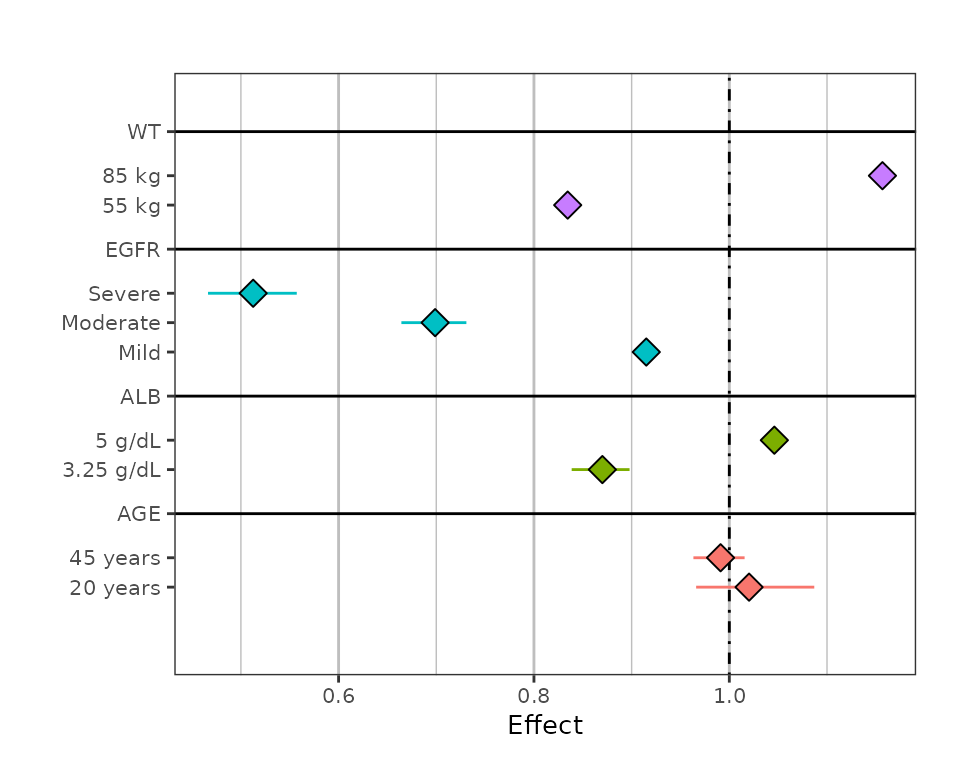
Adding group labels
The summary_labels argument takes a ggplot2::labeller()
function. In this example, we load a list of covariate labels with the
yspec
package and pass it through ggplot2::as_labeller().
spec_file <- yspec::ys_load(
  system.file(file.path("test-data", "spec", "analysis3.yml"), package = "pmforest")
)
all_labels <- yspec::ys_get_short(spec_file, title_case = TRUE)
plot_labels <- as_labeller(unlist(all_labels))

sumData %>%
  plot_forest(vline_intercept = 1,
              summary_label = plot_labels)
Notice the more informative group labels on the y-axis and the CI table,
as compared to the raw values from
Notice the more informative group labels on the y-axis and the CI table,
as compared to the raw values from GROUP shown in the
previous plots.
Adding captions and other labels
This example illustrates the use of the other labelling arguments
(CI_label, x_lab, and
caption).
Some notes:
- The title at the top of the plot (“CL (L/hr)” in the example below)
is pulled from the
metagroupcolumn of the data, as it is most useful when usingmetagroupto make multiple plots (shown later on). Here we just create it withdplyr::mutate()(and add a label for it toplot_labels). -
captionis apatchworkargument. You can change thecaptionformatting usingpatchworkfunctions (see “Patchwork Annotations” section below). - If
CI_labelis not passed, the value passed tox_labwill be used for the table label. -
text_sizeapplies directly toggplotlayers (minimum is 3.5), though the table text will scale with this input accordingly.
all_labels$CL <- 'CL (L/hr)'
plot_labels <- as_labeller(unlist(all_labels))

sumData %>%
  mutate(metagroup = "CL") %>%
  plot_forest(vline_intercept = 1,
              x_lab = "Fraction and 95% CI\nRelative to Reference",
              CI_label = "Median [95% CI]",
              summary_label = plot_labels,
              text_size = 3.5,
              caption = "This is a patchwork caption.
You can add multiple lines.") 
Shaded Interval
You can add a shaded interval over a specified range. It is important
to note that the x-axis is automatically determined based on your input
data. The specified interval may therefore be cut off, as the x limits
do not adjust based on the specified interval. You can correct for this
by specifying the x_breaks and x_limit
arguments.
sumData %>%
  mutate(metagroup = "CL") %>%
  plot_forest(vline_intercept = 1,
              x_lab = "Fraction and 95% CI\nRelative to Reference",
              CI_label = "Median [95% CI]",
              summary_label = plot_labels,
              caption = "This is a patchwork caption.
                         You can add multiple lines.",
              shaded_interval = c(0.8,1.25),
              x_breaks = c(0.4,0.6, 0.8, 1, 1.2, 1.4, 1.6),
x_limit = c(0.6,1.45)) 
Multiple covariates (or facets)
Here we pull in a new dataset with the param column
containing both V2 and CL, where the previous
example only contained CL, and pass this to the
metagroup argument of summarize_data().
sumData2 <- system.file(file.path("test-data", "plotData2.RDS"), package = "pmforest") %>%
  readRDS() %>%
  summarize_data(
    value = stat,
    group = GROUP,
    group_level = LVL,
    metagroup = param
  )
head(sumData2)
#> # A tibble: 6 × 6
#>   group group_level metagroup   mid    lo    hi
#>   <chr> <chr>       <chr>     <dbl> <dbl> <dbl>
#> 1 AGE   20 years    CL        1.02  0.966 1.09
#> 2 AGE   20 years    V2        1     1     1
#> 3 AGE   45 years    CL        0.991 0.963 1.02
#> 4 AGE   45 years    V2        1     1     1
#> 5 ALB   3.25 g/dL   CL        0.870 0.839 0.898
#> 6 ALB   3.25 g/dL   V2        1     1     1
The metagroup argument doesn’t necessarily have to facet
across multiple covariates, though this is a common use case. When doing
this, you may consider setting annotate_CI = FALSE to
simplify the plots.
all_labels$CL <- 'CL (L/hr)'
all_labels$V2 <- 'V (L)'
plot_labels <- as_labeller(unlist(all_labels))

sumData2 %>%
  plot_forest(vline_intercept = 1,
              x_lab = "Fraction and 95% CI\nRelative to Reference",
              CI_label = "Median [95% CI]",
              summary_label = plot_labels,
              caption = "This is a patchwork caption.
                         You can add multiple lines.",
annotate_CI = FALSE) 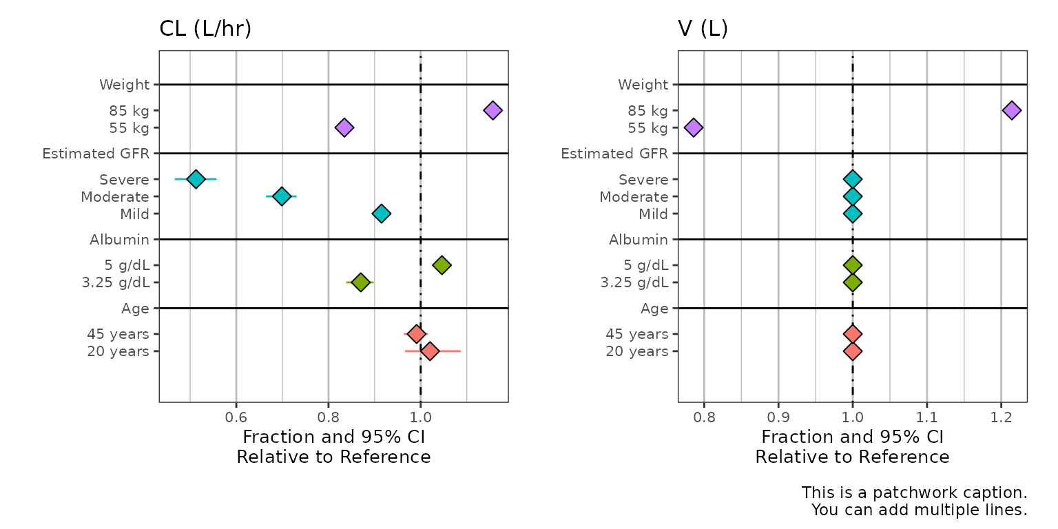
Regardless, you can specify how you want to align the plots using the
nrow argument or other functions in the
patchwork R package.
sumData2 %>%
  plot_forest(vline_intercept = 1,
              x_lab = "Fraction and 95% CI\nRelative to Reference",
              CI_label = "Median [95% CI]",
              summary_label = plot_labels,
              caption = "This is a patchwork caption.
                         You can add multiple lines.",
              plot_width = 9,
nrow = 2) 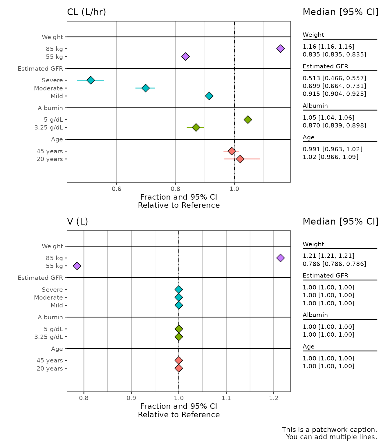
Patchwork Annotations
The individual layers of the returned object are defined using
ggplot, but the final plot is assembled using
patchwork.
Thus you can add additional patchwork themes/annotations
to the returned object, but cannot alter the ggplot layers. Themes can
be added using the & operator, and follow the same
convention as ggplot themes. In this example we change the
formatting of the caption argument, combine the plot with
an example table, and add some additional labels/titles.
clp <- sumData %>%
  mutate(metagroup = "CL") %>%
  plot_forest(vline_intercept = 1,
              x_lab = "Fraction and 95% CI\nRelative to Reference",
              CI_label = "Median [95% CI]",
              summary_label = plot_labels,
              caption = "This is a patchwork caption.
                         You can add multiple lines.")

wrap_plots(clp, grid::textGrob('Text on right side'), widths = c(4,1)) +
  plot_annotation(
    title = 'Here is a title',
    subtitle = 'Here is a subtitle',
    caption = 'Overrides plot_forest caption argument',
    tag_levels = c('A', '1'), tag_prefix = 'Fig. ', tag_sep = '.', tag_suffix = ':',
    theme = theme(plot.title = element_text(size = 18)))  &
  theme(plot.caption = element_text(size = 12),
        plot.tag.position = c(0, 1),
        plot.tag = element_text(size = 8, hjust = 0, vjust = 0))
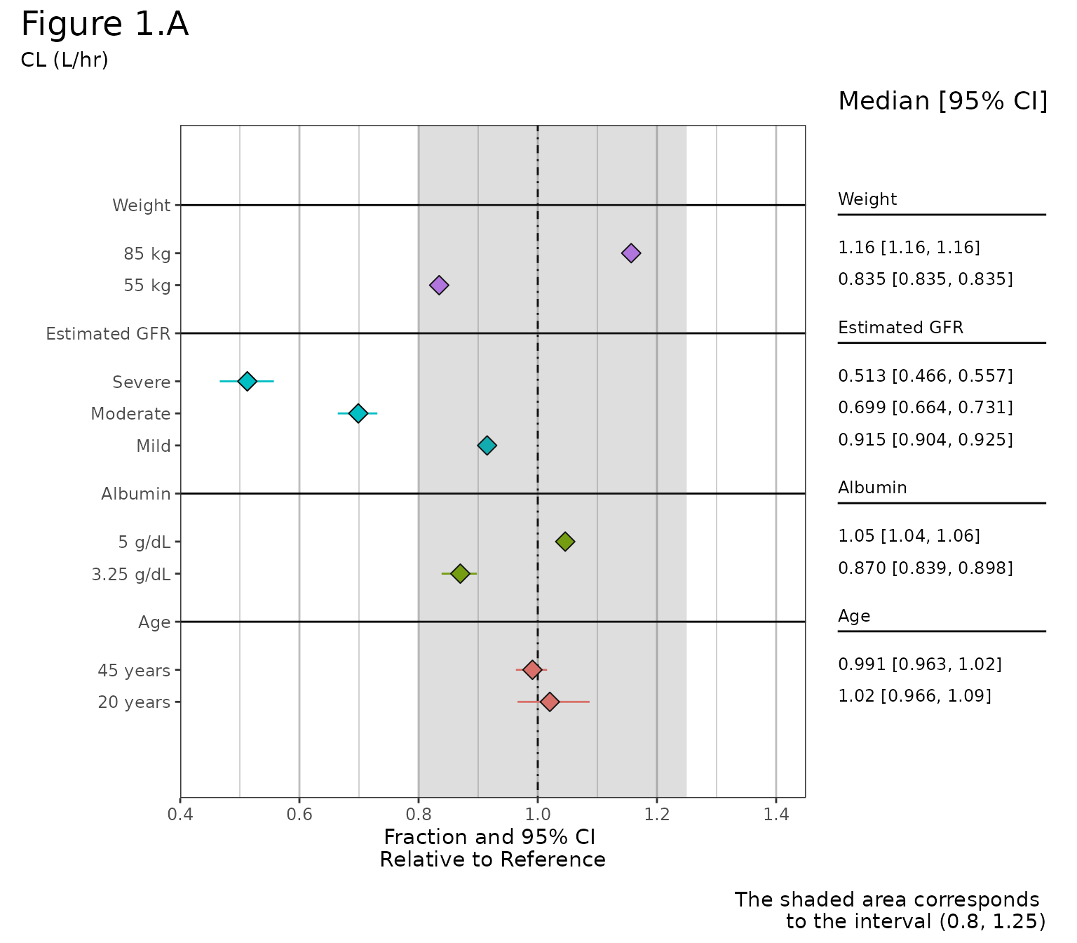
Full Forest Plot Example:
clp <- sumData %>%
          plot_forest(shaded_interval = c(0.8,1.25),
                      summary_label = plot_labels,
                      text_size = 4,
                      vline_intercept = 1,
                      x_lab = "Fraction and 95% CI \nRelative to Reference",
                      CI_label = "Median [95% CI]",
                      caption = "The shaded area corresponds
                                 to the interval (0.8, 1.25)",
                      plot_width = 9, # out of 12
                      x_breaks = c(0.4,0.6, 0.8, 1, 1.2, 1.4),
                      x_limit = c(0.4,1.45),
                      annotate_CI = TRUE)

clp +
    plot_annotation(
          title = 'Figure 1.A',
          subtitle = 'CL (L/hr)',
          theme = theme(plot.title = element_text(size = 18))) &
    theme(plot.caption = element_text(size = 11))