9 Glossary

Users can read in a tex or yaml-formatted glossary file and use those abbreviations and definitions to form table footnotes. The goal is consistency across the project in how terms are defined.

9.1 Create a glossary object

Information from a glossary is stored in a glossary object. The object is a list that contains glossary entries. The glossary object may be created either by reading a glossary file or through a constructor function in R.

9.1.1 Read in a glossary file - TeX

Glossary files can be formatted as a collection of acronyms as you would normally have in a glossary.tex file. Something like this:

\newacronym{AIC}{AIC}{Akaike information criterion}
\newacronym{ALAG}{ALAG}{oral absorption lag time}
\newacronym{ALB}{ALB}{albumin}
\newacronym{ALT}{ALT}{alanine aminotransferase}

Acronyms in TeX glossary files have 3 parts:

1. a label
2. an abbreviation
3. a definition

So the general format for an acronym is

\newacronym{label}{abbreviation}{definition}

In this example,

\newacronym[sort=CLF]{CLF}{CL/F}{apparent clearance}

• CLF is the label
• CL/F is the abbreviation
• apparent clearance is the definition

We read in this glossary file with read_glossary()

glob <- read_glossary("glossary.tex")

head(glob)

. AAG  : alpha-1-acid glycoprotein
. AIC  : Akaike information criterion
. ALAG : oral absorption lag time
. ALB  : albumin
. ALT  : alanine aminotransferase
. AST  : aspartate aminotransferase

When printing the object, you get the label and the abbreviation. To see the full entry, use $ to extract an entry

glob$Cmax

. maximum concentration in the dosing interval (Cmax)

Here, we get the definition and the abbreviation printed to the console.

9.1.2 Read in a glossary file - Yaml

Users can also code their own glossary files in yaml format.

CLF: 
  abb: CL/F
  def: apparent clearance after oral dosing
V2F:
  abb: V2/F
  def: apparent central volume of distribution
QF:
  abb: Q/F
  def: apparent intercompartmental clearance
V3F:
  abb: V3/F
  def: apparent peripheral volume of distribution

For this format,

1. Put the label in the outer level (e.g., CLF or V2F)
2. Put the abbreviation under abb
3. Put the definition under def

We can read the glossary file in yaml format again with read_glossary()

yam <- read_glossary("glossary.yaml")

yam

. CLF : apparent clearance after oral dosing
. V2F : apparent central volume of distribution
. QF  : apparent intercompartmental clearance
. V3F : apparent peripheral volume of distributi...

9.1.3 Create with R constructor

Use the as_glossary() function to create a glossary object in your R session

glo <- as_glossary(a = "apple", b = "banana", g = "grape")

glo

. a : apple
. b : banana
. g : grape

Alternatively, you can coerce a list

l <- list(a = "apple", b = "banana", g = "grape")

glo <- as_glossary(l)

In this object, the label and the abbreviation are assumed to be the same.

glo$g

. grape (g)

To update the abbreviation,

glo <- update_abbrev(glo, g = "gr")

glo$g

. grape (gr)

9.2 Create table notes

Once the glossary object is created, you can form table notes using the glossary_notes() function.

Pass in the glossary object and the unquoted names you want to select out of the glossary

glossary_notes(glob, WT, ALB) 

. [1] "WT: weight; ALB: albumin"

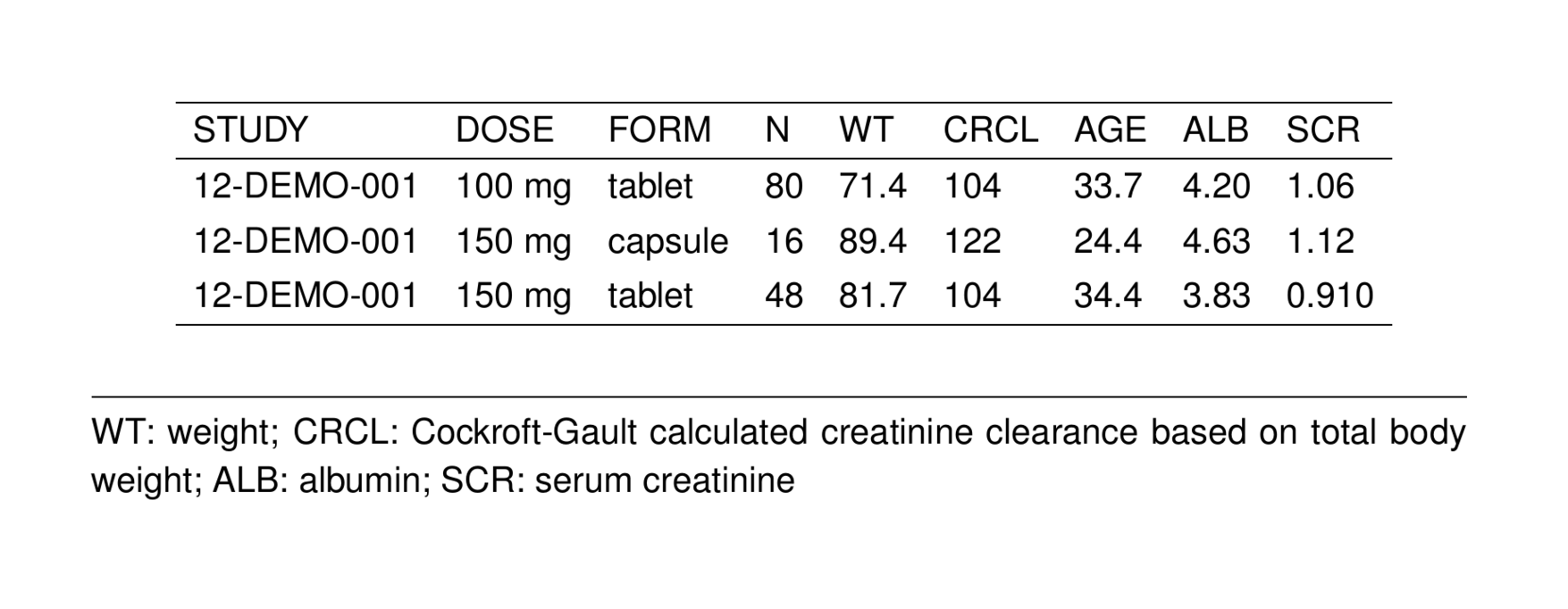
This generates a ;-separated string with abbreviation: definition format for all the entries you selected. This can be added to a table as notes:

notes <- glossary_notes(glob, WT, ALB, SCR)

st_new(stdata()[1:3,]) %>% 
  st_notes(notes) %>% 
  stable() %>% 
  st_as_image()

9.2.1 Inline

Notes can also be attached to a table inline with st_notes_glo()

st_new(stdata()[1:3,]) %>% 
  st_notes_glo(glob, WT, CRCL, ALB, SCR) %>% 
  stable() %>% 
  st_as_image()

Notice in this example that the notes are longer than the longest line in the table and the formatting looks off. In this case, use the width argument to detach the notes into a minipage arrangement

st_new(stdata()[1:3,]) %>% 
  st_notes_glo(glob, WT, CRCL, ALB, SCR, width = 0.9) %>% 
  stable() %>% 
  st_as_image()

9.3 Work with glossary objects

9.3.1 Update the abbreviation

glob$hl

. elimination half-life (\ensuremath{t_{1/2}})

glob <- update_abbrev(glob, hl = "t1/2")

glob$hl

. elimination half-life (t1/2)

9.3.2 Update the definition

There is no api to update the definition. This change should be made in the glossary file.

9.3.3 Select certain items in a glossary object

glob2 <- select_glossary(glob, AIC, BIC)

glob2

. AIC : Akaike information criterion
. BIC : Bayesian information criterion

9.3.4 Combine two glossary objects

Use the c function.

glob3 <- c(glob2, glo)

glob3

. AIC : Akaike information criterion
. BIC : Bayesian information criterion
. a   : apple
. b   : banana
. g   : grape

The labels in the objects you are combining must be unique. You will get an error if you try combining two objects which contain the same label

x <- glo
y <- as_glossary(m = "mango", b = "blueberry")
try(c(x,y))

. Error in c.glossary(x, y) : Arguments cannot share any names.

In this case you can drop the duplicate name from one of the objects

intersect(names(x), names(y))

. [1] "b"

z <- select_glossary(glo, -b)

z

. a : apple
. g : grape

c(z, y)

. a : apple
. g : grape
. m : mango
. b : blueberry

9.3.5 Get the glossary as a plain R list

as.list(glob)[1]

. $AAG
. $AAG$abbreviation
. [1] "AAG"
. 
. $AAG$definition
. [1] "alpha-1-acid glycoprotein"

9.3.6 Get the glossary object as a data frame

as.data.frame(glo)

.   label definition abbreviation
. 1     a      apple            a
. 2     b     banana            b
. 3     g      grape           gr

9.3.7 View the glossary object

You’ll have to coerce to data frame first

View(as.data.frame(glo))

9.3.8 Extract one glossary entry

glo$a

. apple (a)

or

glo[["a"]]

. apple (a)

9.3.9 Extract multiple glossary entries

select_glossary(glo, a, g)

. a : apple
. g : grape

or

glo[c("b", "g")]

. b : banana
. g : grape

9.3.10 Extract the abbreviations

purrr::map(glob, "abbreviation")[1:2]

. $AAG
. [1] "AAG"
. 
. $AIC
. [1] "AIC"

9.3.11 Extract the definitions

purrr::map(glob, "definition")[1:2]

. $AAG
. [1] "alpha-1-acid glycoprotein"
. 
. $AIC
. [1] "Akaike information criterion"