9 pmtable

Some setup

Please see the yspec package.

units <- yspec::ys_get_unit(
  yspec::ys_help$spec(), 
  parens = TRUE
)

Data sets that come with pmtables; we’ll re-name them for later

data <- pmt_first
data_pk <- pmt_pk
data_all <- pmt_obs

9.1 Principles

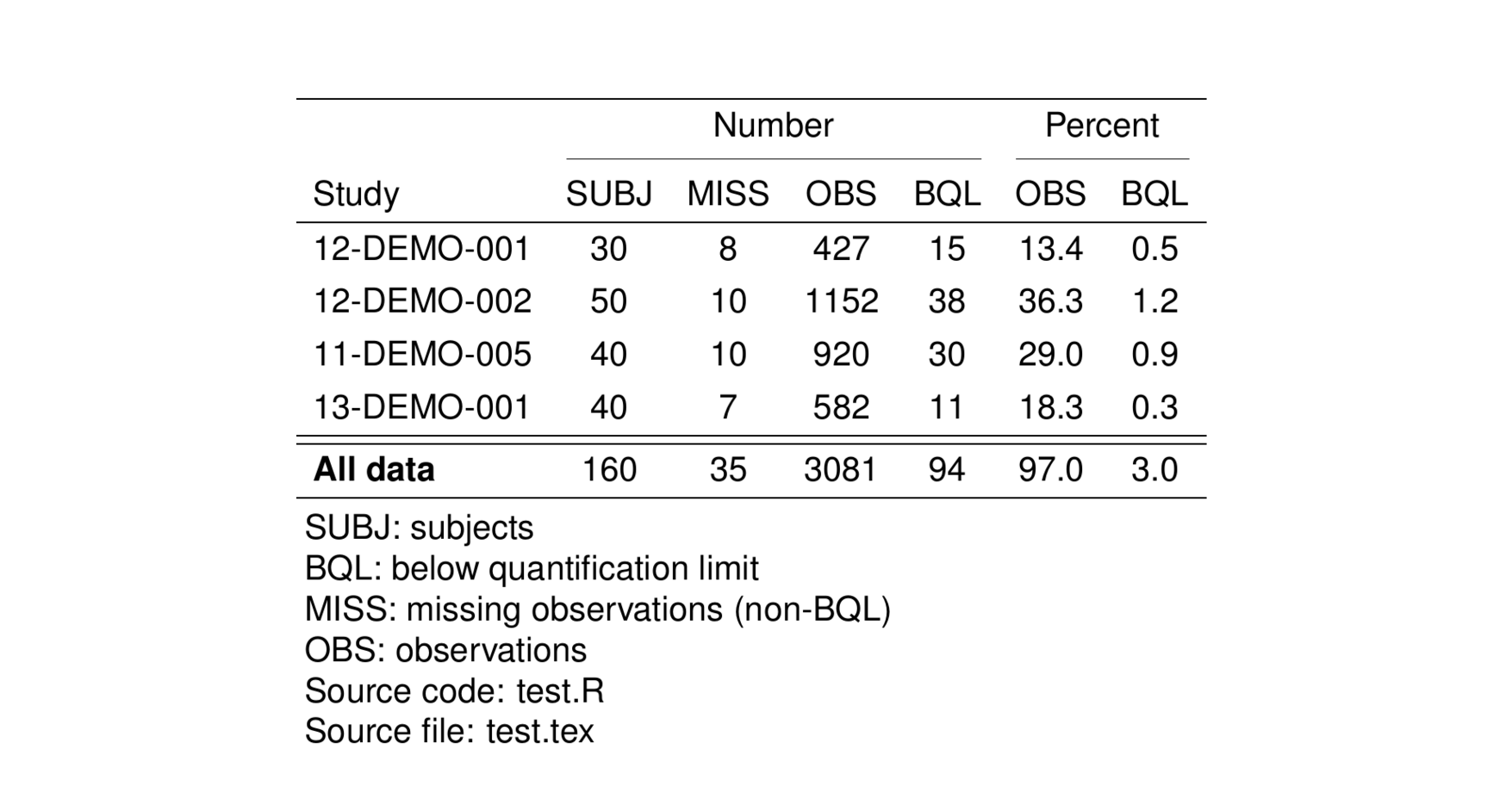
These functions expect that the user passes in all data that is to be summarized and nothing more. We will not filter your data.

9.2 Rename cols

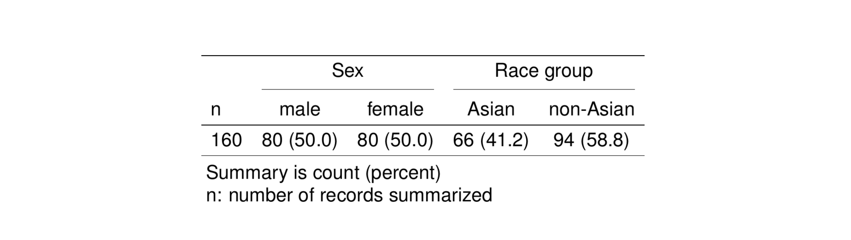
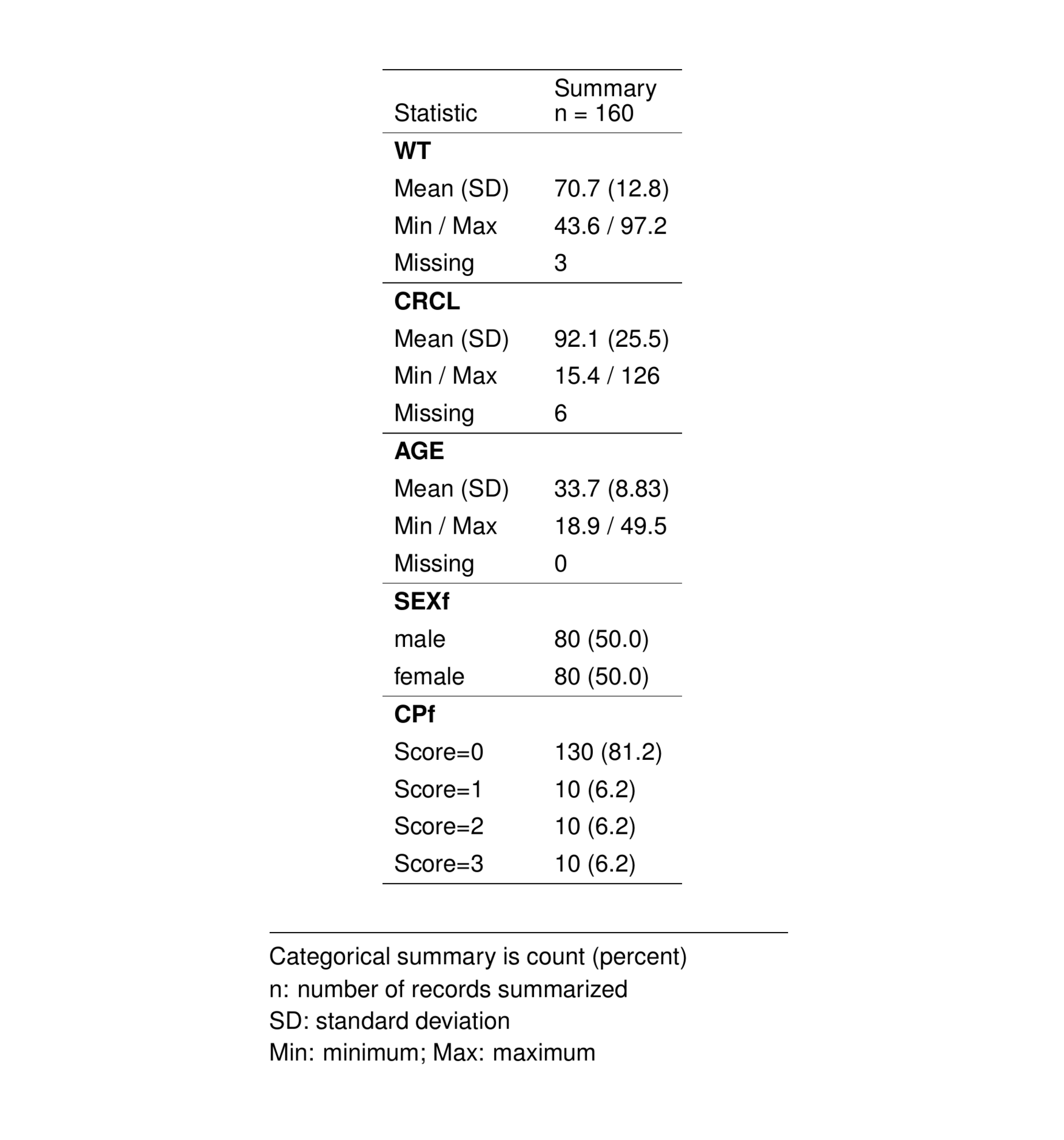
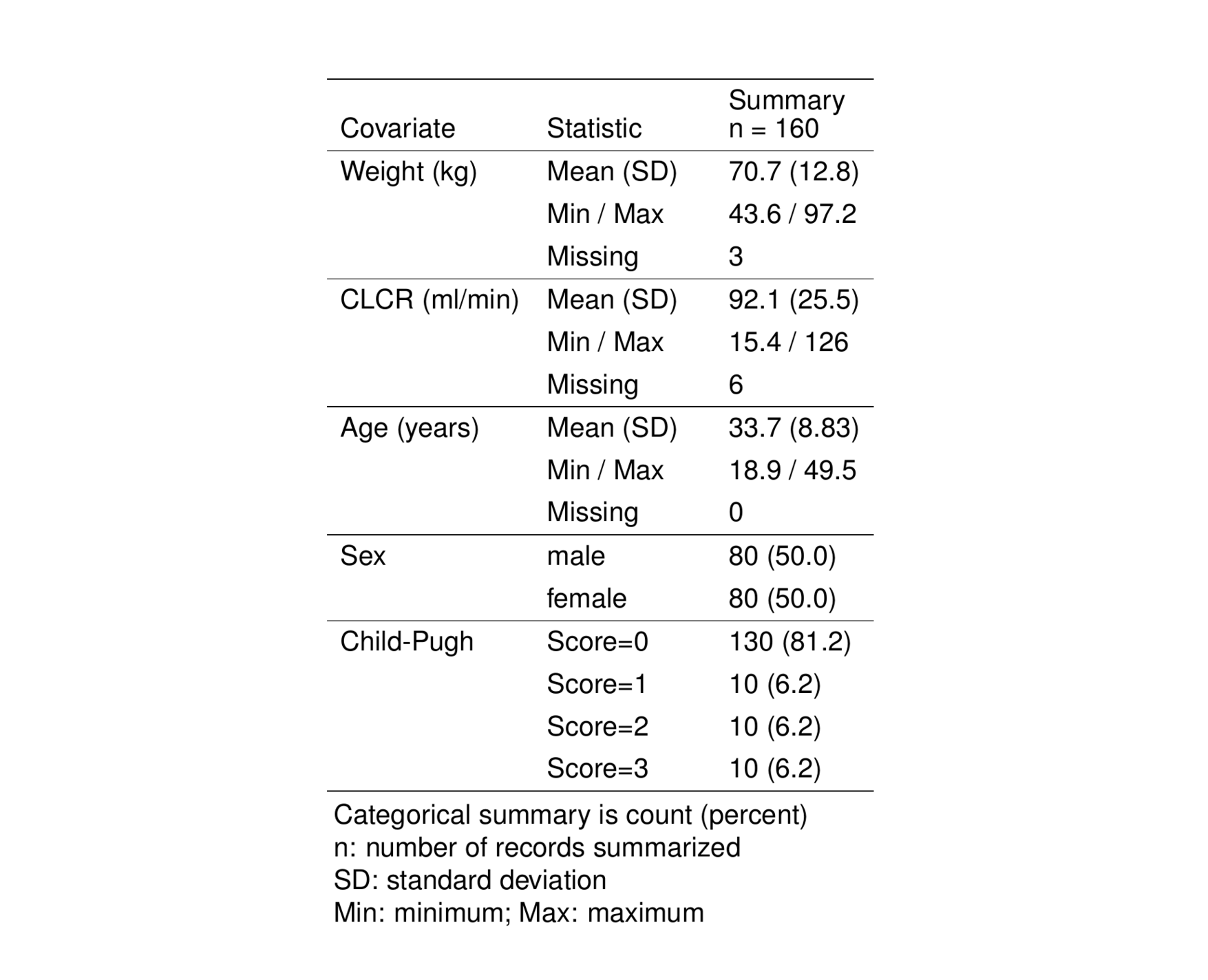
When you select columns to summarize, you can generally pass in alternate (nicer) names that you want to show up in the table. For example, if I have a column called WT in the data frame and I want it to show up as Weight this can be accomplished during the call

pt_cont_wide(data, cols = c(Weight = "WT")) %>% 
  stable(notes = NULL) %>% 
  st_as_image()

Alternatively, you can use the table argument to enter rename info. Note that table is a list that should have names that match up with columns in the data frame and values that are the new names

tab <- list(SEXf = "Sex", ASIANf = "Race group")

pt_cat_wide(data, cols = "SEXf,ASIANf", table = tab) %>% 
  stable() %>% 
  st_as_image()

9.3 Data inventory tables

• Count number of
• individuals
• observations
• BQL observations
• missing values
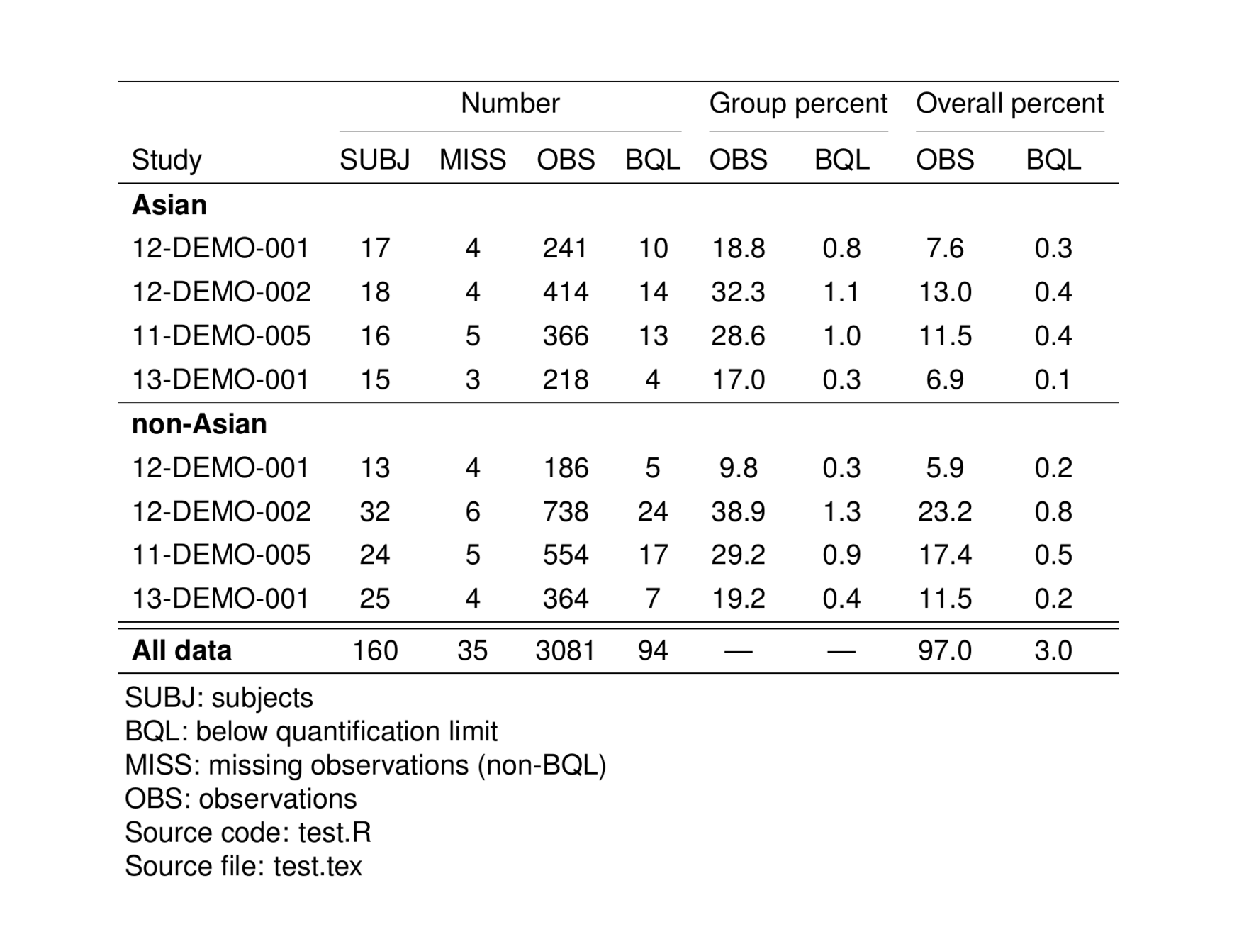
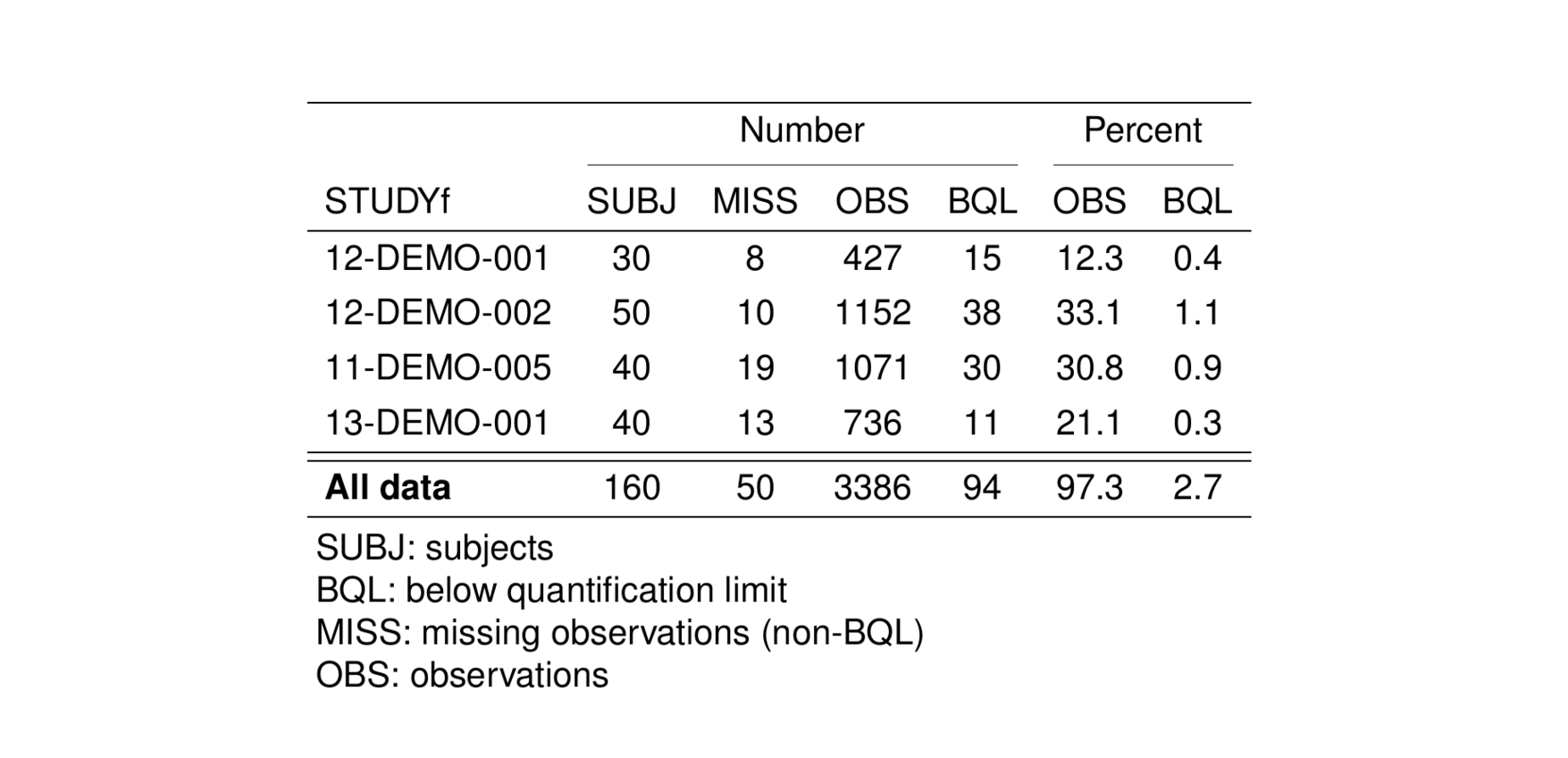
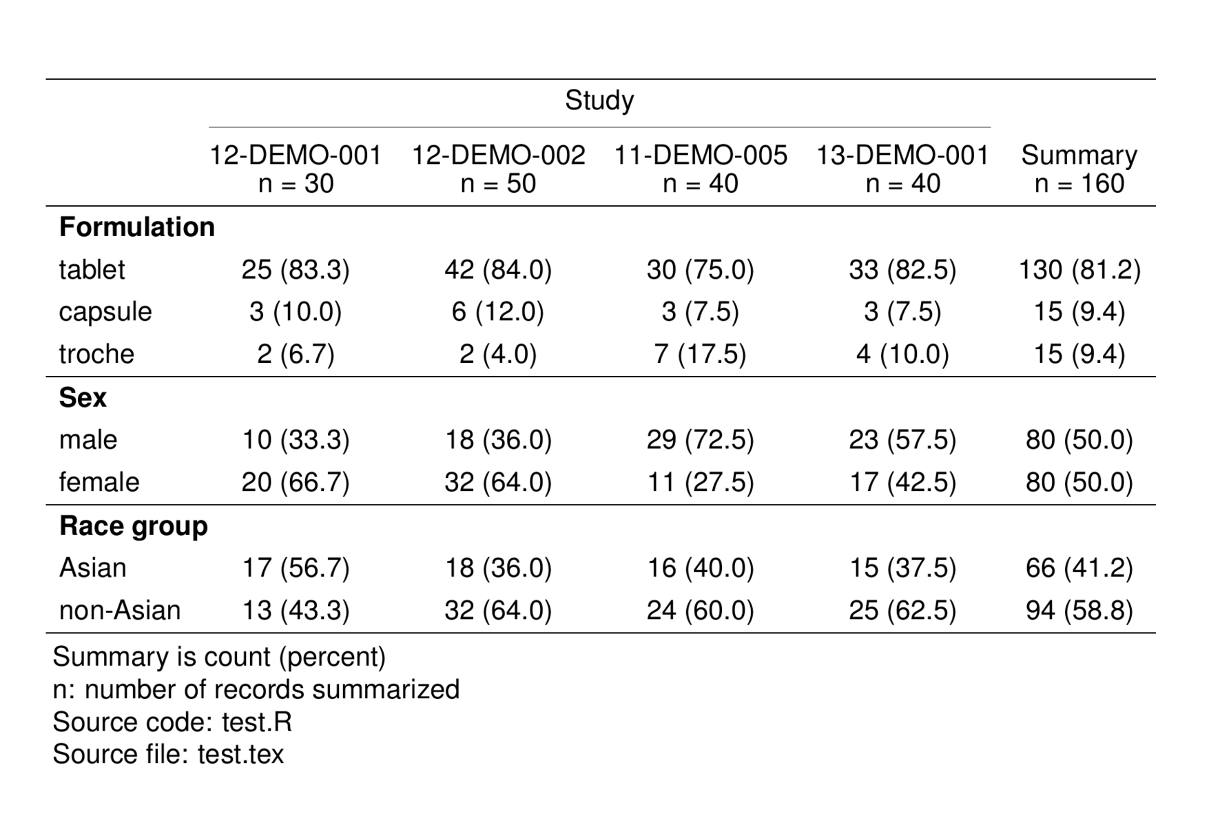
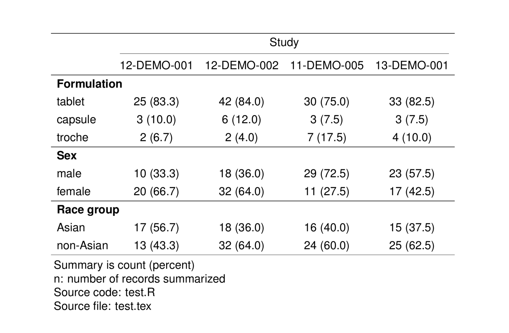
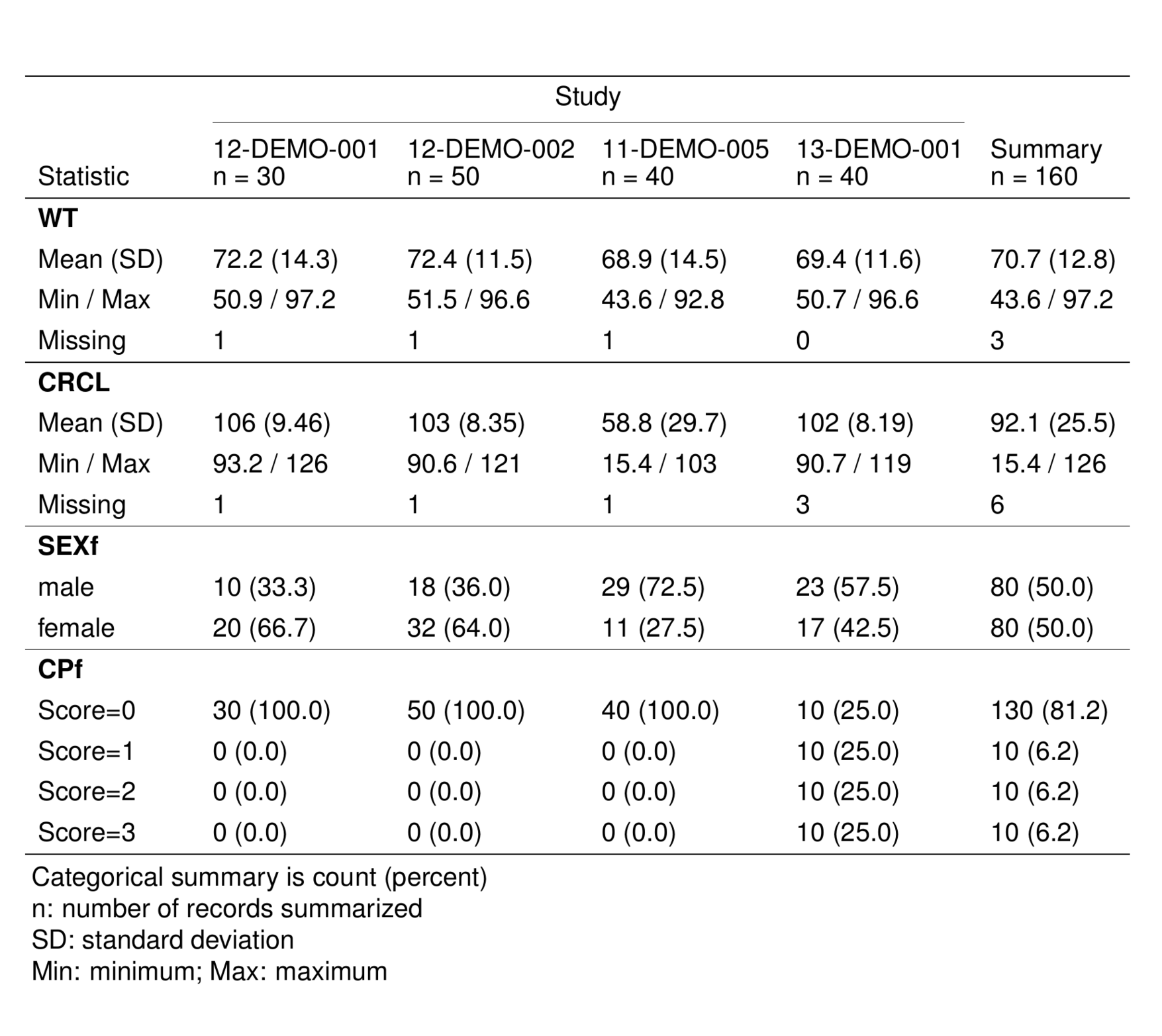
• Calculate the percent of observations or BQL in different sub groups

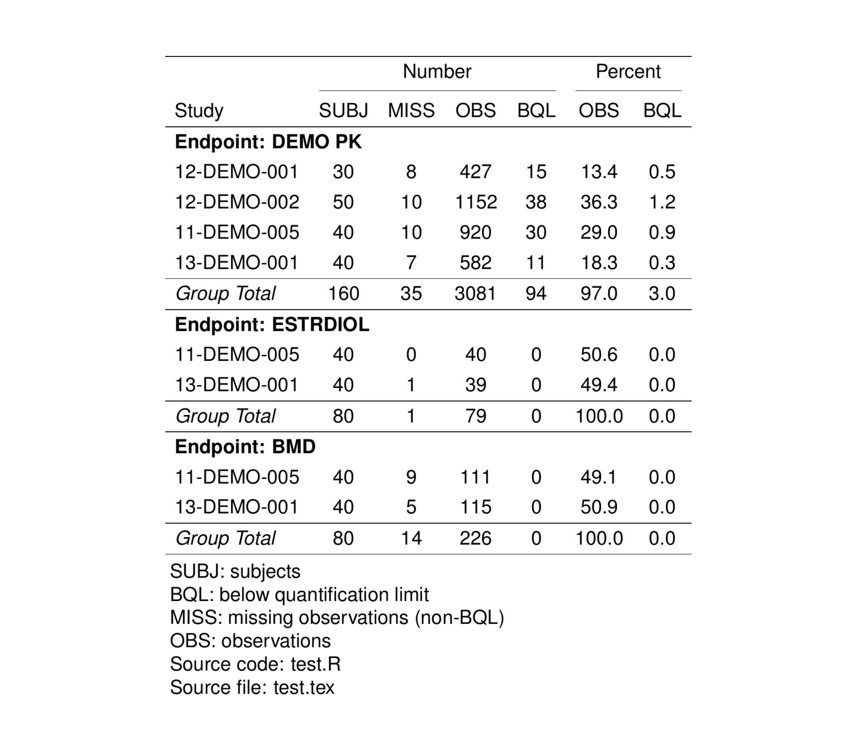
9.3.1 Stacked by endpoint

• The stacked plot creates multiple independent tables to summarize different endpoints; there is no single overall summary for the table because we are summarizing different endpoints

out <- pt_data_inventory(
  data_all,
  by = c(Study = "STUDYf"),
  panel = as.panel("SEQf", prefix = "Endpoint: "),
  stacked = TRUE
)

stable(
  out, 
  r_file = "test.R", 
  output_file = "test.tex"
) %>% st_as_image()

9.3.2 Paneled

• Just summarize a single endpoint

out <- pt_data_inventory(
  data_pk,
  by = c(Study = "STUDYf"),
  panel = "ASIANf"
)

stable(
  out, 
  r_file = "test.R", 
  output_file = "test.tex"
) %>% st_as_image()

9.3.3 Grouped (by study)

out <- pt_data_inventory(
  data_pk,
  by = c(Study = "STUDYf")
)

stable(
  out, 
  r_file = "test.R", 
  output_file = "test.tex"
) %>% st_as_image()

9.3.4 BQL / BLQ

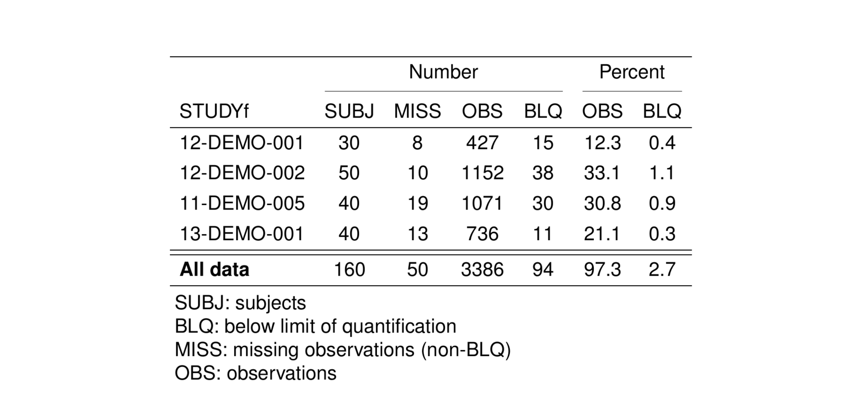
Beginning with version 0.4.1, pmtables can accommodate either BQL or BLQ as the name of the column indicating that observations were below the limit of quantitation. Table notes and output column headers will be adjusted based on the input.

For example

data_ql <- pmt_obs
data_lq <- rename(pmt_obs, BLQ = BQL) 

pt_data_inventory(data_ql, by = "STUDYf") %>% 
  stable() %>%
  st_as_image()

pt_data_inventory(data_lq, by = "STUDYf") %>% 
  stable() %>%
  st_as_image()

9.4 Wide categorical table

• Summary of categorical data in wide format
• The summary is number (percent within group)
• Wide refers to the fact that the covariates go across the table

9.4.0.1 Ungrouped

out <- pt_cat_wide(
  data = data,
  cols = vars(Formulation = FORMf, Sex = SEXf, "Race group" = ASIANf)
)

stable(
  out, 
  r_file = "test.R", 
  output_file = "test.tex"
) %>% st_as_image()

9.4.1 Paneled (limited utility, IMO)

• Provided here for completeness

out <- pt_cat_wide(
  data = data,
  cols = vars(Formulation = FORMf, Sex = SEXf, "Race group" = ASIANf),
  panel = as.panel("STUDYf", prefix = "Study: ")
)

stable(
  out, 
  r_file = "test.R", 
  output_file = "test.tex"
) %>% st_as_image()

9.4.2 Grouped (by male / female)

out <- pt_cat_wide(
  data = data,
  by = c(Sex = "SEXf"),
  cols = vars(Formulation = FORMf, "Race group" = ASIANf)
)

stable(
  out, 
  r_file = "test.R", 
  output_file = "test.tex"
) %>% st_as_image()

9.4.3 Paneled and grouped

out <- pt_cat_wide(
  data = data,
  cols = vars(Formulation = FORMf, Sex = SEXf, "Race group" = ASIANf),
  panel = as.panel("STUDYf", prefix = "Study: "),
  by = c("RF Group" = "RFf")
)

stable(
  out, 
  r_file = "test.R", 
  output_file = "test.tex"
) %>% st_as_image()

9.4.4 No summary

out <- pt_cat_wide(
  data = data,
  summarize = "none",
  cols = vars(Formulation = FORMf, Sex = SEXf, "Race group" = ASIANf),
  panel = as.panel("STUDYf", prefix = "Study: "),
  by = c("RF Group" = "RFf")
)

stable(
  out, 
  r_file = "test.R", 
  output_file = "test.tex"
) %>% st_as_image()

9.5 Long categorical table

• Categorical table in long format
• Long indicates that the covariates go down the table

9.5.1 Ungrouped

out <- pt_cat_long(
  data = data,
  cols = vars(Study = STUDYf, Sex = SEXf, "Race group" = ASIANf, "Child-Pugh" = CPf)
)

stable(
  out, 
  r_file = "test.R", 
  output_file = "test.tex"
) %>% st_as_image()

9.5.2 Grouped (by formulation)

out <- pt_cat_long(
  data = data,
  cols = vars(Study = STUDYf, Sex = SEXf, "Race group" = ASIANf, "Child-Pugh" = CPf),
  span = c(Formulation = "FORMf")
)

stable(
  out, 
  r_file = "test.R", 
  output_file = "test.tex"
) %>% st_as_image()

9.5.3 Summary on bottom and right

out <- pt_cat_long(
  data = data,
  summarize = "both",
  cols = vars(Formulation = FORMf, Sex = SEXf, "Race group" = ASIANf),
  span = vars(Study = STUDYf)
)

stable(
  out, 
  r_file = "test.R", 
  output_file = "test.tex"
) %>% st_as_image()

9.5.4 No summary

out <- pt_cat_long(
  data = data,
  summarize = "none",
  cols = vars(Formulation = FORMf, Sex = SEXf, "Race group" = ASIANf),
  span = vars(Study = STUDYf)
)

stable(
  out, 
  r_file = "test.R", 
  output_file = "test.tex"
) %>% st_as_image()

9.6 Wide continuous table

• Continuous table in wide format
• Wide means that the covariates go across the table

9.6.1 Ungrouped

out <- pt_cont_wide(
  data = data,
  cols = "WT,SCR,AGE,ALB,HT",
  units = units
)

stable(
  out, 
  r_file = "test.R", 
  output_file = "test.tex"
) %>% st_as_image()

9.6.2 Paneled

out <- pt_cont_wide(
  data = data,
  cols = "WT,SCR,AGE,ALB,HT",
  panel = c(Study = "STUDYf"),
  units = units
)

stable(
  out, 
  r_file = "test.R", 
  output_file = "test.tex"
) %>% st_as_image()

9.6.3 Grouped (by study)

out <- pt_cont_wide(
  data = data,
  cols = "WT,SCR,AGE,ALB",
  by = c(Study = "STUDYf"),
  units = units
)

stable(
  out, 
  r_file = "test.R", 
  output_file = "test.tex"
) %>% st_as_image()

9.6.4 Paneled and grouped

out <- pt_cont_wide(
  data = data,
  cols = "WT,SCR,AGE,ALB",
  by = c(Study = "STUDYf"),
  panel = c(Formulation = "FORMf"),
  units = units
)

stable(
  out, 
  r_file = "test.R", 
  output_file = "test.tex"
) %>% st_as_image()

9.7 Long continuous table

• Continuous summary table in long format
• Long indicates that covariates go down the table

9.7.1 Ungrouped

out <- pt_cont_long(
  data = data,
  cols = "WT,SCR,AGE",
  units = units
)

stable(
  out, 
  r_file = "test.R", 
  output_file = "test.tex"
) %>% st_as_image()

9.7.2 Paneled

out <- pt_cont_long(
  data = data,
  cols = "WT,SCR,AGE",
  panel = vars(Study = STUDYf),
  units = units
)

stable(
  out, 
  r_file = "test.R", 
  output_file = "test.tex"
) %>% st_as_image()

9.8 Demographics table

A demographics table summarizes both continuous and discrete data in a single table.

• Both continuous columns (cols_cont) and discrete (cols_cat) are required
• You can specify a span column (the table is pretty skinny without that)
• You can opt out of the paneling too with paneled argument (the also makes the table wider
• An All data summary is provided on the left (opt out with summarize_all)

9.8.1 With span

pt_demographics(
  pmt_first, 
  cols_cont = "WT, CRCL", 
  cols_cat = "SEXf, CPf", 
  span = c(Study = "STUDYf")
) %>% stable() %>% st_as_image()

9.8.2 No span

• This table is skinny

mini <- noteconf(type = "minipage", width = 0.5)

pt_demographics(
  pmt_first, 
  cols_cont = "WT, CRCL, AGE", 
  cols_cat = "SEXf, CPf"
) %>% stable(note_config = mini) %>% st_as_image()

9.8.3 No span, not paneled

• Opting out of the paneling also makes it wider

pt_demographics(
  pmt_first, 
  cols_cont = "WT, CRCL, AGE", 
  cols_cat = "SEXf, CPf", 
  paneled = FALSE, 
  table = list(
    WT   = "Weight (kg)", 
    CRCL = "CLCR (ml/min)", 
    AGE  = "Age (years)", 
    SEXf = "Sex", 
    CPf  = "Child-Pugh"
  )
) %>% stable() %>% st_as_image()

9.8.4 No summary

pt_demographics(
  pmt_first, 
  cols_cont = "WT, CRCL, AGE", 
  cols_cat = "SEXf, CPf", 
  span = c(Study = "STUDYf"),
  summarize_all = FALSE
) %>% stable() %>% st_as_image()

9.9 Customized summary functions

pmtables will summarize continuous data using a built-in function, producing standard summaries (e.g. mean, median, etc). Users can pass a function to replace this default, allowing totally customized summaries.

Custom summary functions are not currently allowed for categorical data.

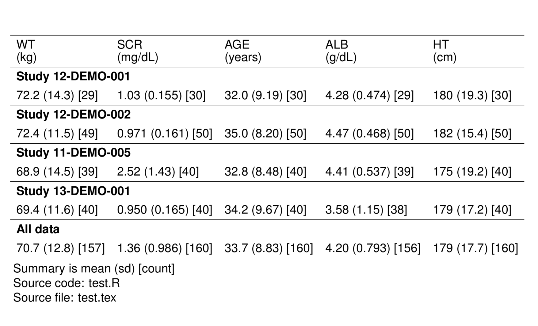
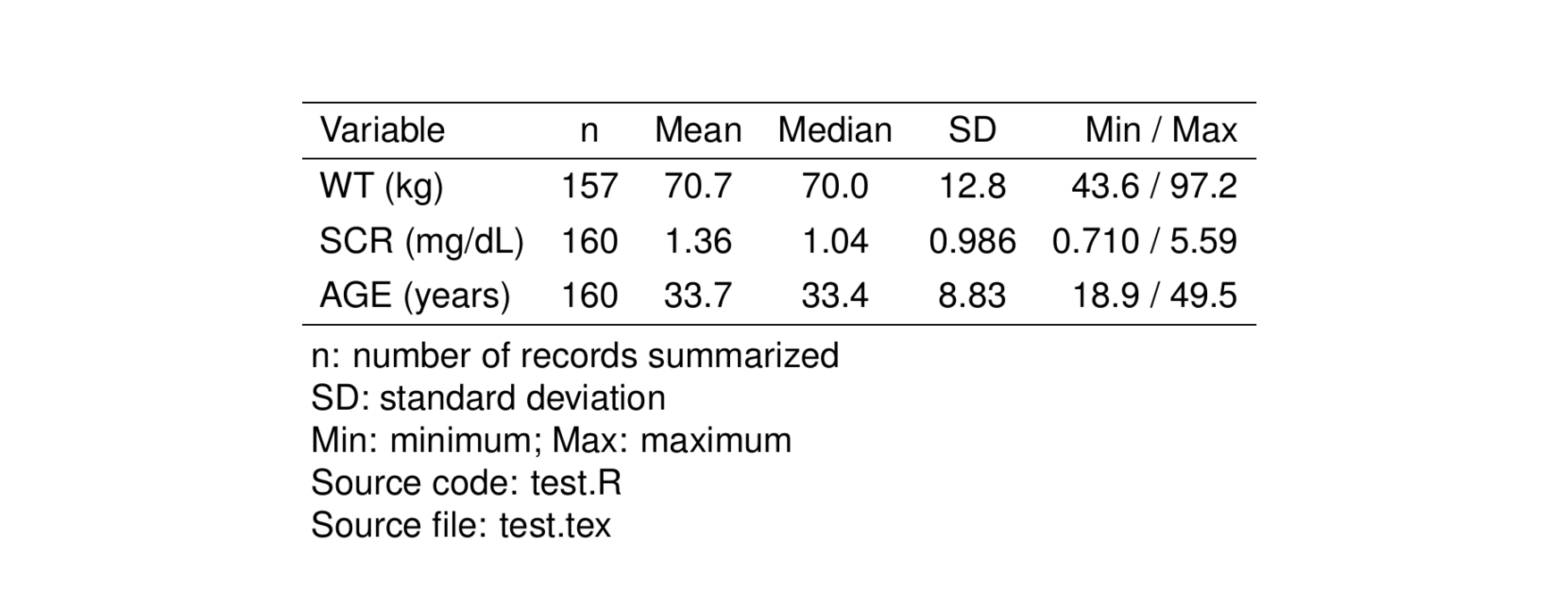
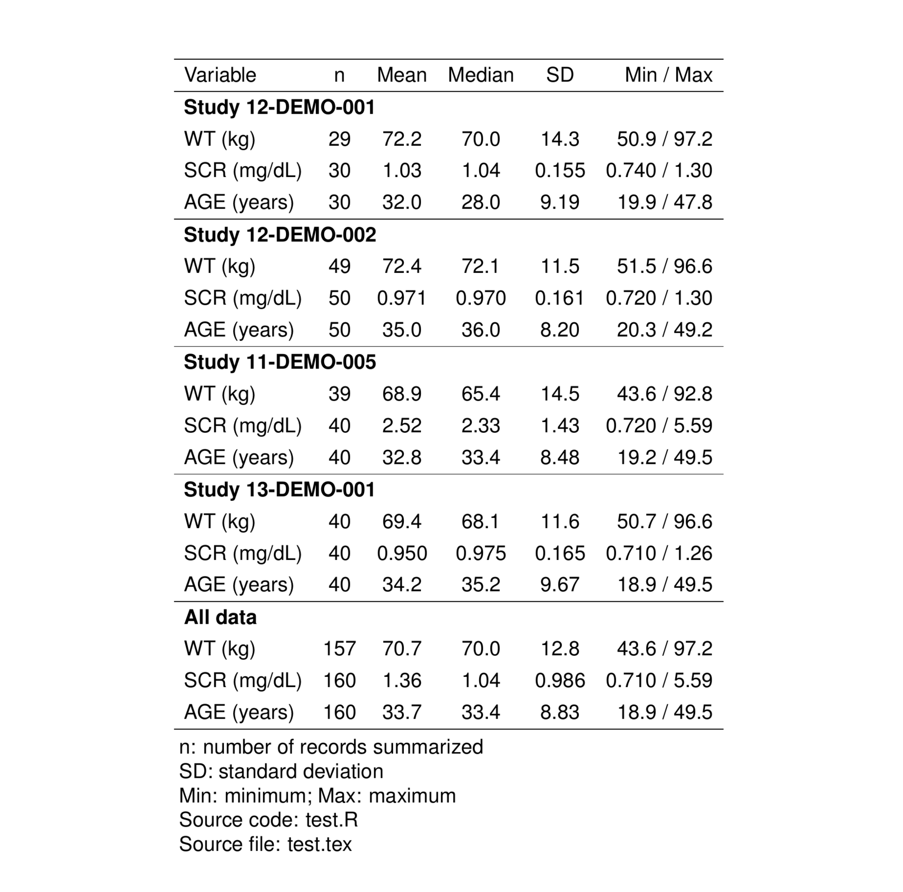
9.9.1 Continuous long table

You can pass a custom summary function via fun. This function should have a first argument called value and should be able to absorb extra arguments via .... The function should return a data.frame, with a single row and summaries going across in the columns.

For example, we can have pt_cont_long() return the geometric mean and variance by passing the following function

cont_long_custom <- function(value, ...) {
  value <- na.omit(value)
  ans <- data.frame(
    GeoMean = exp(mean(log(value))), 
    Variance = var(value)
  )
  mutate(ans, across(everything(), sig))
}

Test the function by passing some test data

cont_long_custom(c(1,2,3,4,5))

  GeoMean Variance
1    2.61     2.50

Then, pass this as fun

pt_cont_long(
  data = pmt_first, 
  cols = c("WT", "ALB", "AGE"), 
  fun = cont_long_custom
)$data

# A tibble: 3 × 3
  Variable GeoMean Variance
  <chr>    <chr>   <chr>   
1 WT       69.5    165     
2 ALB      4.11    0.629   
3 AGE      32.5    78.0    

See pmtables:::cont_long_fun (the default) for an example.

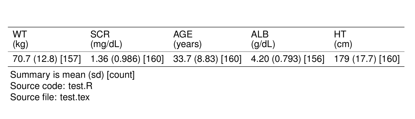
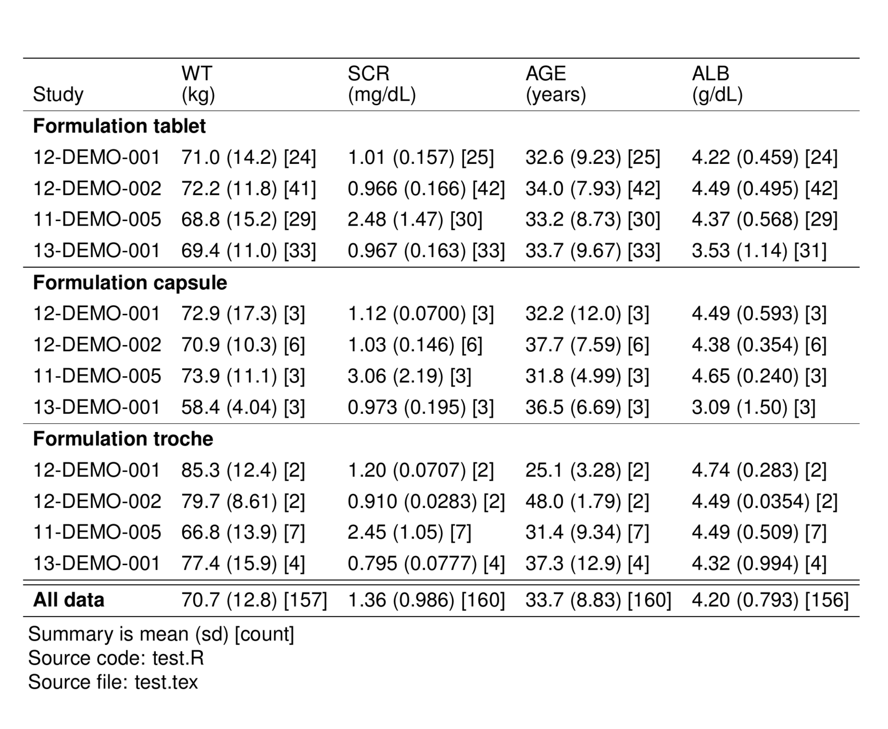
9.9.2 Continuous wide table

You can pass a custom summary function via fun. This function should have a first argument called value and should be able to absorb extra arguments via .... The continuous, wide table must return a data.frame with a single row and a single column named summary

cont_wide_custom <- function(value, ...) {
  value <- na.omit(value)
  geo_mean <- sig(exp(mean(log(value))))
  variance <- sig(var(value))
  n <- length(value)
  ans <- paste0(geo_mean, " [", variance, "] (", n, ")")
  data.frame(summary = ans)
}

You can test the function by passing some test data

cont_wide_custom(c(1, 3, 5))

          summary
1 2.47 [4.00] (3)

Then, pass this as fun

pt_cont_wide(
  data = pmt_first, 
  cols = c("WT", "ALB", "AGE"), 
  fun = cont_wide_custom
)$data

# A tibble: 1 × 3
  WT               ALB                AGE              
  <chr>            <chr>              <chr>            
1 69.5 [165] (157) 4.11 [0.629] (156) 32.5 [78.0] (160)

See pmtables:::cont_wide_fun (the default) for an example.