4 Spanners

4.1 Syntax

Set the span argument to the output of as.span(). The key arguments for as.span() are the spanner title and the names of the columns over which you want the spanner to run

stable(
  stdata(), 
  span = as.span("Covariates", WT:SCR)
)

The equivalent pipe syntax is

st_new(stdata()) %>% 
  st_span("Covariates", WT:SCR)

4.2 Basics

A column spanner puts a horizontal line over a sequence of column names and places a title above that line forming a column group.

As a trivial example:

data <- 
  tibble(
    Tariffville = "06081",  
    Connecticut= "CT", 
    Minnesota = "MN", 
    Minneapolis = "55455"
  ) 

stable(
  data, 
  span = as.span("States", Connecticut:Minnesota)
) %>%  st_as_image()

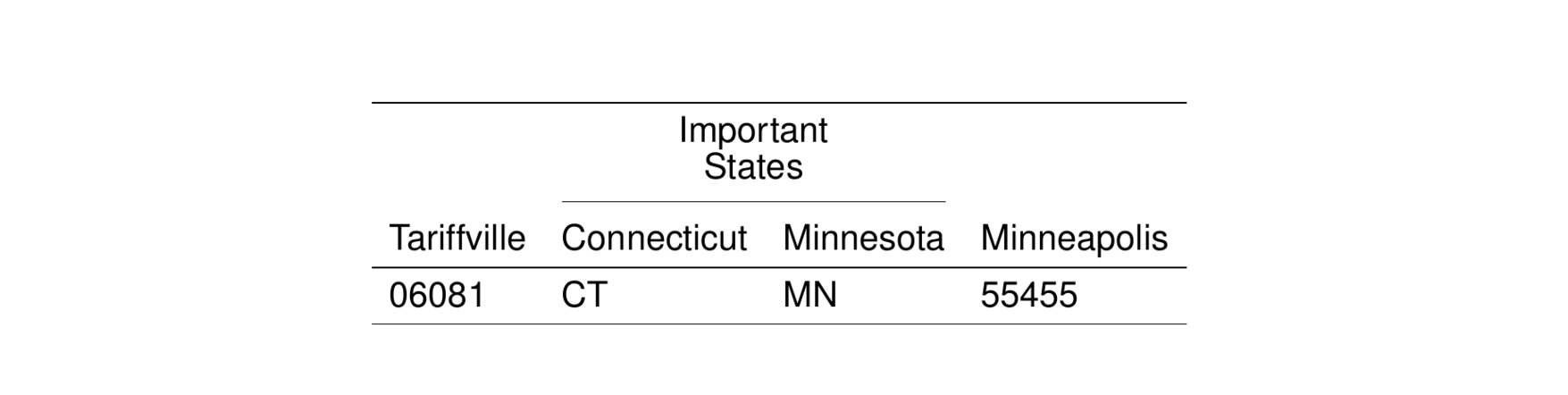
4.3 Multiple spanners

Multiple spanners can be added to a table by specifying the level for any spanner that you want to be placed above the lowest level spanner. For example,

sp <- list(
  as.span("States", Connecticut:Minnesota), 
  as.span("Important Locations", Tariffville:Minneapolis, level = 2)
)

stable(data, span = sp) %>% 
  st_as_image()

Note that to specify multiple spanners, we pass a list of span objects. I’ve simplified the code a bit here by creating that list as a standalone object and then passing the whole list as span.

4.3.1 Using pipe syntax

For problems like this, it might be preferable to use the pipe syntax

data %>%
  st_new() %>% 
  st_span("States", Connecticut:Minnesota) %>% 
  st_span("Important Locations", Tariffville:Minneapolis, level = 2) %>% 
  stable() %>% 
  st_as_image()

4.4 Breaking span title

We can make the title of the span break across multiple lines by using ...

stable(
  data, 
  span = as.span("Important ... States", Connecticut:Minnesota)) %>%
  st_as_image()

4.5 Aligning span title

Beginning with version 0.4.1, the span title can be left or right justified in addition to the default centering

stable(
  stdata(), 
  span = as.span("Covariates", WT:SCR, align = 'l')
) %>% st_as_image()

4.6 Span created by splitting column names

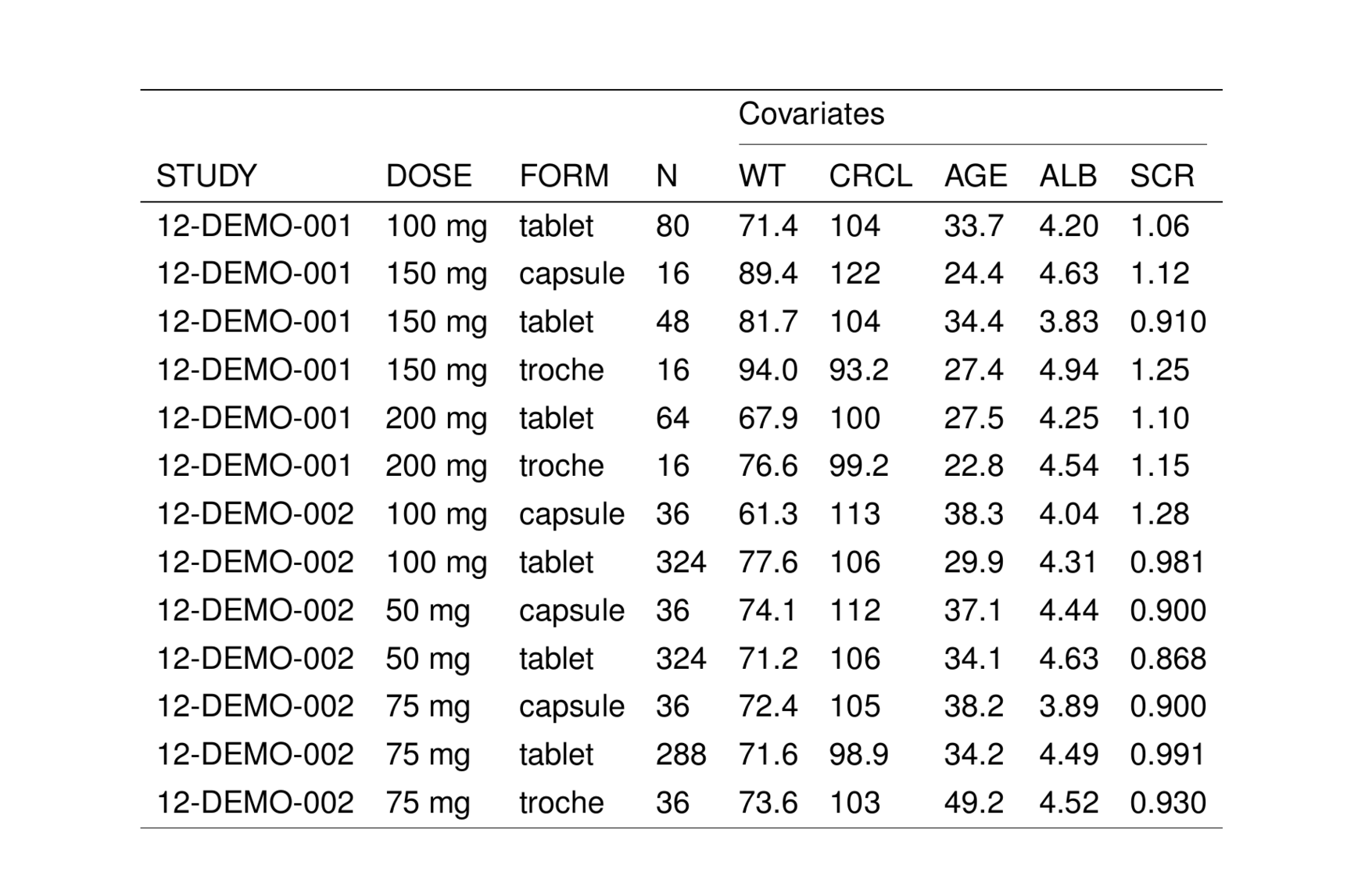
colsplit() is a way to create column spanners which are encoded into the column names of the input data frame; the names are split on a separator character (like .) and either the left or right side are taken as the title and the other is taken as the column name.

Consider this data

  A.first A.second B.third B.fourth
1       1        2       3        4

Notice the natural grouping between A.first and A.second; we want first and second grouped together with the title A. Similar setup for third and fourth under the title B.

We can make table with spanners by passing a call to colsplit() as span_split

stable(dd, span_split = colsplit(sep = '.')) %>% 
  st_as_image()

4.6.1 pivot_longer workflow

This is pattern is convenient when summarizing data in a long format. To to demonstrate, we’ll calculate summary statistics for WT and AGE by STUDY

summ <- 
  pmt_first %>%
  pivot_longer(cols = c("WT", "AGE")) %>% 
  filter(!is.na(value)) %>%
  group_by(STUDYf, name) %>% 
  summarise(Mean = mean(value), Sd = sd(value), N = n(), .groups = "drop") %>%
  mutate(across(Mean:N, sig)) %>% 
  mutate(across(Mean:N, as.character))

summ

# A tibble: 8 × 5
  STUDYf      name  Mean  Sd    N    
  <fct>       <chr> <chr> <chr> <chr>
1 12-DEMO-001 AGE   32.0  9.19  30   
2 12-DEMO-001 WT    72.2  14.3  29   
3 12-DEMO-002 AGE   35.0  8.20  50   
4 12-DEMO-002 WT    72.4  11.5  49   
5 11-DEMO-005 AGE   32.8  8.48  40   
6 11-DEMO-005 WT    68.9  14.5  39   
7 13-DEMO-001 AGE   34.2  9.67  40   
8 13-DEMO-001 WT    69.4  11.6  40   

Now take 2 (or 3) more steps to get the table in the right shape to feed into stable(). First, pivot this longer using the summary stat name

long <- pivot_longer(summ, cols = c("Mean", "Sd", "N"), names_to = "stat")
head(long)

# A tibble: 6 × 4
  STUDYf      name  stat  value
  <fct>       <chr> <chr> <chr>
1 12-DEMO-001 AGE   Mean  32.0 
2 12-DEMO-001 AGE   Sd    9.19 
3 12-DEMO-001 AGE   N     30   
4 12-DEMO-001 WT    Mean  72.2 
5 12-DEMO-001 WT    Sd    14.3 
6 12-DEMO-001 WT    N     29   

Second, we’ll make name more appealing / informative

long <- mutate(
  long, 
  name = recode(name, WT = "Weight (kg)", AGE = "Age (years)")
)

Third, pivot this wider using the covariate name and stat

wide <- pivot_wider(
  long, 
  names_from = c("name", "stat"), 
  names_sep = "---"
)
wide

# A tibble: 4 × 7
  STUDYf     `Age (years)--…` `Age (years)--…` `Age (years)--…` `Weight (kg)--…`
  <fct>      <chr>            <chr>            <chr>            <chr>           
1 12-DEMO-0… 32.0             9.19             30               72.2            
2 12-DEMO-0… 35.0             8.20             50               72.4            
3 11-DEMO-0… 32.8             8.48             40               68.9            
4 13-DEMO-0… 34.2             9.67             40               69.4            
# … with 2 more variables: `Weight (kg)---Sd` <chr>, `Weight (kg)---N` <chr>

Now we have column names set up to create the spanners

stable(wide, span_split = colsplit(sep = "---")) %>% 
  st_as_image()

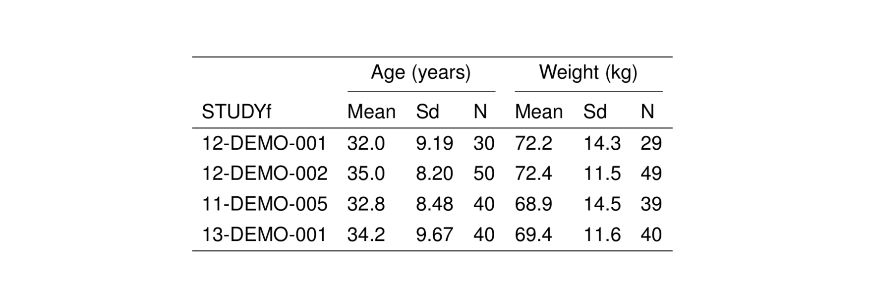
This workflow takes several steps to complete, but once you identify the pattern it can be just an extra step or two beyond what you’re already doing to get a nice table.