Effect Compartment Population Model
Here we expand the Two-compartment model for single patient to a population model fitted to the combined data from phase I and phase IIa studies. The parameters exhibit inter-individual variations (IIV), due to both random effects and to the patients' body weight, treated as a covariate and denoted \(bw\).
1 Population Model for Plasma Drug Concentration \(c\)
\begin{gather*}
\log\left(c_{ij}\right) \sim N\left(\log\left(\widehat{c}_{ij}\right),\sigma^2\right), \\\
\widehat{c}_{ij} = f_{2cpt}\left(t_{ij},D_j,\tau_j,CL_j,Q_j,V_{1j},V_{2j},k_{aj}\right), \\\
\log\left(CL_j,Q_j,V_{ssj},k_{aj}\right) \sim N\left(\log\left(\widehat{CL}\left(\frac{bw_j}{70}\right)^{0.75},\widehat{Q}\left(\frac{bw_j}{70}\right)^{0.75}, \widehat{V}_{ss}\left(\frac{bw_j}{70}\right),\widehat{k}_a\right),\Omega\right), \\\
V_{1j} = f_{V_1}V_{ssj}, \\\
V_{2j} = \left(1 - f_{V_1}\right)V_{ssj}, \\\
\left(\widehat{CL},\widehat{Q},\widehat{V}_{ss},\widehat{k}_a, f_{V_1}\right) = \left(10\ {\rm L/h},15\ {\rm L/h},140\ {\rm L},2\ {\rm h^{-1}}, 0.25 \right), \\\
\Omega = \left(\begin{array}{cccc} 0.25^2 & 0 & 0 & 0 \ 0 & 0.25^2 & 0 & 0 \\\
0 & 0 & 0.25^2 & 0 \ 0 & 0 & 0 & 0.25^2 \end{array}\right), \\\
\sigma = 0.1
\end{gather*}
Furthermore we add a fourth compartment in which we measure a PD effect(Figure 1).
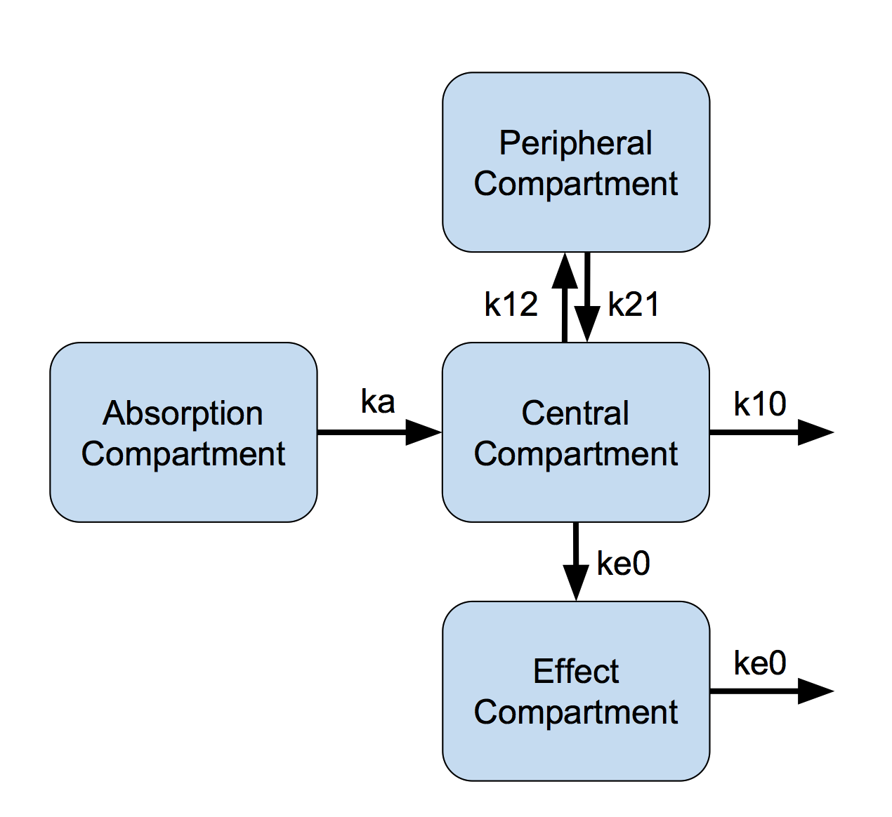
Figure 1: Effect Compartment Model
2 Effect Compartment Model for PD response \(R\).
\begin{gather*}
R_{ij} \sim N\left(\widehat{R}_{ij},\sigma_{R}^2\right), \\\
\widehat{R}_{ij} = \frac{E_{max}c_{eij}}{EC_{50j} + c_{eij}}, \\\
c_{e\cdot j}^\prime = k_{e0j}\left(c_{\cdot j} - c_{e\cdot j}\right), \\\
\log\left(EC_{50j}, k_{e0j}\right) \sim N\left(\log\left(\widehat{EC}_{50}, \widehat{k}_{e0}\right),\Omega_R\right), \\\
\left(E_{max}, \widehat{EC}_{50},\widehat{k}_{e0}\right) = \left(100, 100.7, 1\right), \\\
\Omega_R = \left(\begin{array}{cc} 0.2^2 & 0 \ 0 & 0.25^2 \end{array}\right), \ \ \ \sigma_R = 10.
\end{gather*}
The PK and the PD data are simulated using the following treatment.
- Phase I study
- Single dose and multiple doses
- Parallel dose escalation design
- 25 subjects per dose
- Single doses: 5, 10, 20, and 40 mg
- PK: plasma concentration of parent drug (\(c\))
- PD response: Emax function of effect compartment concentration (\(R\))
- PK and PD measured at 0.125, 0.25, 0.5, 0.75, 1, 2, 3, 4, 6, 8, 12, 18, and 24 hours
- Phase IIa trial in patients
- 100 subjects
- Multiple doses: 20 mg
- sparse PK and PD data (3-6 samples per patient)
The model is simultaneously fitted to the PK and the PD
data. For this effect compartment model, we construct a
constant rate matrix and use pmx_solve_linode. Correct use of
Torsten requires the user pass the entire event history
(observation and dosing events) for an individual to the
function. Thus the Stan model shows the call to pmx_solve_linode
within a loop over the individual subjects rather than over
the individual observations. Note that the correlation matrix \(\rho\) does not explicitly appear
in the model, but it is used to construct \(\Omega\), which parametrizes
the PK IIV.
data{
  int<lower = 1> nSubjects;
  int<lower = 1> nt;
  int<lower = 1> nObs;
  int<lower = 1> iObs[nObs];
  real<lower = 0> amt[nt];
  int<lower = 1> cmt[nt];
  int<lower = 0> evid[nt];
  int<lower = 1> start[nSubjects];
  int<lower = 1> end[nSubjects];
  real<lower = 0> time[nt];
  vector<lower = 0>[nObs] cObs;
  vector[nObs] respObs;
  real<lower = 0> weight[nSubjects];
  real<lower = 0> rate[nt];
  real<lower = 0> ii[nt];
  int<lower = 0> addl[nt];
  int<lower = 0> ss[nt];
}

transformed data{
  vector[nObs] logCObs = log(cObs);
  int<lower = 1> nRandom = 5;
  int nCmt = 4;
  real biovar[nCmt] = rep_array(1.0, nCmt);
  real tlag[nCmt] = rep_array(0.0, nCmt);
}

parameters{
  real<lower = 0> CLHat;
  real<lower = 0> QHat;
  real<lower = 0> V1Hat;
  real<lower = 0> V2Hat;
  //  real<lower = 0> kaHat;
  real<lower = (CLHat / V1Hat + QHat / V1Hat + QHat / V2Hat +
                sqrt((CLHat / V1Hat + QHat / V1Hat + QHat / V2Hat)^2 -
                     4 * CLHat / V1Hat * QHat / V2Hat)) / 2> kaHat; // ka > lambda_1
  real<lower = 0> ke0Hat;
  real<lower = 0> EC50Hat;
  vector<lower = 0>[nRandom] omega;
  corr_matrix[nRandom] rho;
  real<lower = 0> omegaKe0;
  real<lower = 0> omegaEC50;
  real<lower = 0> sigma;
  real<lower = 0> sigmaResp;

  // reparameterization
  vector[nRandom] logtheta_raw[nSubjects];
  real logKe0_raw[nSubjects];
  real logEC50_raw[nSubjects];
}

transformed parameters{
  vector<lower = 0>[nRandom] thetaHat;
  cov_matrix[nRandom] Omega;
  real<lower = 0> CL[nSubjects];
  real<lower = 0> Q[nSubjects];
  real<lower = 0> V1[nSubjects];
  real<lower = 0> V2[nSubjects];
  real<lower = 0> ka[nSubjects];
  real<lower = 0> ke0[nSubjects];
  real<lower = 0> EC50[nSubjects];
  matrix[nCmt, nCmt] K;
  real k10;
  real k12;
  real k21;
  row_vector<lower = 0>[nt] cHat;
  row_vector<lower = 0>[nObs] cHatObs;
  row_vector<lower = 0>[nt] respHat;
  row_vector<lower = 0>[nObs] respHatObs;
  row_vector<lower = 0>[nt] ceHat;
  matrix[nCmt, nt] x;

  matrix[nRandom, nRandom] L;
  vector[nRandom] logtheta[nSubjects];
  real logKe0[nSubjects];
  real logEC50[nSubjects];

  thetaHat[1] = CLHat;
  thetaHat[2] = QHat;
  thetaHat[3] = V1Hat;
  thetaHat[4] = V2Hat;
  thetaHat[5] = kaHat;

  Omega = quad_form_diag(rho, omega); // diag_matrix(omega) * rho * diag_matrix(omega)
  L = cholesky_decompose(Omega);

  for(j in 1:nSubjects){
    logtheta[j] = log(thetaHat) + L * logtheta_raw[j];
    logKe0[j] = log(ke0Hat) + logKe0_raw[j] * omegaKe0;
    logEC50[j] = log(EC50Hat) + logEC50_raw[j] * omegaEC50;

    CL[j] = exp(logtheta[j, 1]) * (weight[j] / 70)^0.75;
    Q[j] = exp(logtheta[j, 2]) * (weight[j] / 70)^0.75;
    V1[j] = exp(logtheta[j, 3]) * weight[j] / 70;
    V2[j] = exp(logtheta[j, 4]) * weight[j] / 70;
    ka[j] = exp(logtheta[j, 5]);
    ke0[j] = exp(logKe0[j]);
    EC50[j] = exp(logEC50[j]);

    k10 = CL[j] / V1[j];
    k12 = Q[j] / V1[j];
    k21 = Q[j] / V2[j];

    K = rep_matrix(0, nCmt, nCmt);

    K[1, 1] = -ka[j];
    K[2, 1] = ka[j];
    K[2, 2] = -(k10 + k12);
    K[2, 3] = k21;
    K[3, 2] = k12;
    K[3, 3] = -k21;
    K[4, 2] = ke0[j];
    K[4, 4] = -ke0[j];

    x[, start[j]:end[j] ] = pmx_solve_linode(time[start[j]:end[j]], amt[start[j]:end[j]],
                                             rate[start[j]:end[j]], ii[start[j]:end[j]],
                                             evid[start[j]:end[j]], cmt[start[j]:end[j]],
                                             addl[start[j]:end[j]], ss[start[j]:end[j]], K, biovar, tlag);

    cHat[start[j]:end[j]] = 1000 * x[2, start[j]:end[j]] ./ V1[j];
    ceHat[start[j]:end[j]] = 1000 * x[4, start[j]:end[j]] ./ V1[j];
    respHat[start[j]:end[j]] = 100 * ceHat[start[j]:end[j]] ./
       (EC50[j] + ceHat[start[j]:end[j]]);
  }

  cHatObs = cHat[iObs];
  respHatObs = respHat[iObs];
}

model{
  // Prior
  CLHat ~ lognormal(log(10), 0.2);
  QHat ~ lognormal(log(15), 0.2);
  V1Hat ~ lognormal(log(30), 0.2);
  V2Hat ~ lognormal(log(100), 0.2);
  kaHat ~ lognormal(log(5), 0.25);
  ke0Hat ~ lognormal(log(10), 0.25);
  EC50Hat ~ lognormal(log(1.0), 0.2);
  omega ~ normal(0, 0.2);
3 Results
We use the same diagnosis tools as for the
previous examples. Table 1 summarises the
statistics and diagnostics of the parameters. In particular, rhat
for all parameters being close to 1.0 indicates convergence of the 4
chains. Figure 2 shows the posterior density of
the parameters.
Posterior prediction check (PPC) in Figure 3 - 7 show that the fits to the plasma concentration are in close agreement with the data, notably for the sparse data case (phase IIa study). The fits to the PD data (Figure 8 - 12) look reasonable considering data being more noisy so the model produces larger credible intervals. Both the summary table and PPC plots show that the estimated values of the parameters are consistent with the values used to simulate the data.
| variable | mean | median | sd | mad | q5 | q95 | rhat | ess_bulk | ess_tail |
|---|---|---|---|---|---|---|---|---|---|
| CLHat | 10.121 | 10.120 | 0.195 | 0.192 | 9.797 | 10.445 | 1.007 | 319.942 | 630.619 |
| QHat | 14.858 | 14.853 | 0.347 | 0.344 | 14.301 | 15.432 | 1.000 | 1106.126 | 1712.821 |
| V1Hat | 34.493 | 34.516 | 1.004 | 0.995 | 32.814 | 36.086 | 1.004 | 671.777 | 1563.396 |
| V2Hat | 103.269 | 103.291 | 2.876 | 2.878 | 98.568 | 108.019 | 1.002 | 1689.165 | 2580.382 |
| kaHat | 1.968 | 1.969 | 0.076 | 0.074 | 1.843 | 2.087 | 1.001 | 1204.531 | 1747.427 |
| ke0Hat | 1.102 | 1.100 | 0.046 | 0.045 | 1.030 | 1.180 | 1.001 | 4008.337 | 3167.030 |
| EC50Hat | 99.512 | 99.542 | 2.124 | 2.098 | 95.981 | 102.987 | 1.000 | 2557.436 | 2773.519 |
| omega[1] | 0.268 | 0.267 | 0.016 | 0.016 | 0.242 | 0.295 | 1.008 | 594.842 | 978.297 |
| omega[2] | 0.229 | 0.228 | 0.021 | 0.021 | 0.195 | 0.264 | 1.002 | 1245.453 | 1966.911 |
| omega[3] | 0.212 | 0.211 | 0.029 | 0.029 | 0.165 | 0.261 | 1.005 | 623.820 | 1692.248 |
| omega[4] | 0.263 | 0.262 | 0.026 | 0.026 | 0.221 | 0.306 | 1.002 | 1396.611 | 2260.425 |
| omega[5] | 0.272 | 0.271 | 0.036 | 0.035 | 0.217 | 0.335 | 1.008 | 293.132 | 728.867 |
| rho[1,2] | 0.197 | 0.200 | 0.100 | 0.101 | 0.029 | 0.360 | 1.003 | 1322.261 | 1955.862 |
| rho[1,3] | -0.161 | -0.161 | 0.122 | 0.121 | -0.361 | 0.042 | 1.001 | 1609.160 | 2270.515 |
| rho[1,4] | -0.101 | -0.105 | 0.107 | 0.107 | -0.270 | 0.083 | 1.001 | 1685.591 | 2353.498 |
| rho[1,5] | 0.016 | 0.015 | 0.128 | 0.128 | -0.192 | 0.226 | 1.000 | 2039.767 | 2939.988 |
| rho[2,3] | 0.091 | 0.092 | 0.144 | 0.148 | -0.143 | 0.328 | 1.008 | 718.187 | 1550.836 |
| rho[2,4] | 0.186 | 0.190 | 0.125 | 0.125 | -0.025 | 0.384 | 1.005 | 948.704 | 1819.199 |
| rho[2,5] | 0.146 | 0.145 | 0.157 | 0.161 | -0.111 | 0.402 | 1.003 | 626.620 | 1546.157 |
| rho[3,4] | 0.815 | 0.827 | 0.093 | 0.094 | 0.646 | 0.947 | 1.010 | 309.098 | 736.635 |
| rho[3,5] | -0.318 | -0.323 | 0.219 | 0.228 | -0.678 | 0.055 | 1.016 | 200.806 | 607.958 |
| rho[4,5] | -0.295 | -0.299 | 0.161 | 0.162 | -0.551 | -0.019 | 1.008 | 546.998 | 1151.092 |
| omegaKe0 | 0.265 | 0.265 | 0.047 | 0.047 | 0.188 | 0.346 | 1.001 | 1731.276 | 2049.892 |
| omegaEC50 | 0.216 | 0.216 | 0.020 | 0.020 | 0.182 | 0.249 | 1.001 | 1599.567 | 1844.056 |
| sigma | 0.099 | 0.099 | 0.002 | 0.002 | 0.095 | 0.103 | 1.002 | 1726.283 | 2836.027 |
| sigmaResp | 10.165 | 10.166 | 0.198 | 0.198 | 9.844 | 10.495 | 1.002 | 4788.527 | 2923.203 |
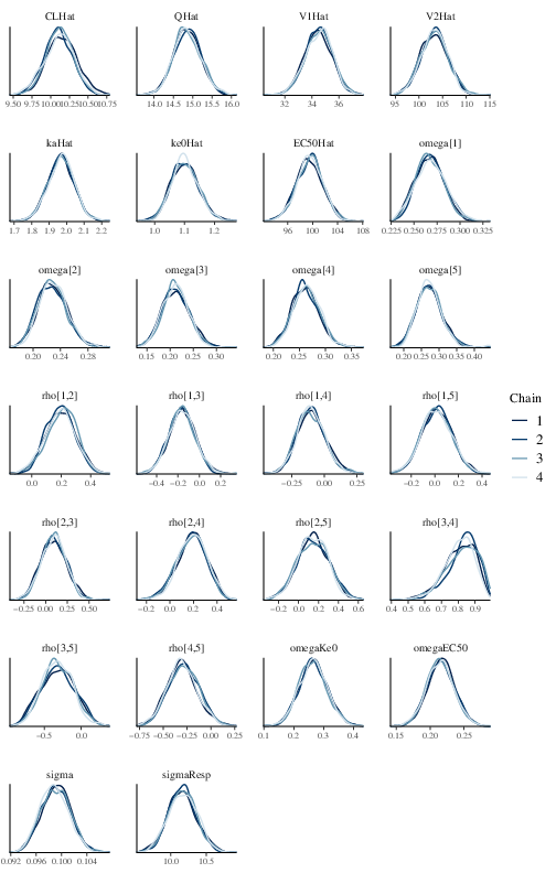
Figure 2: Posterior marginal densities of the model parameters of the effect compartment model.
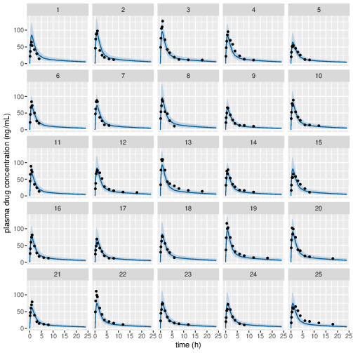
Figure 3: Predicted (90% credible interval and median) and observed individual plasma drug concentrations in study 1 (5mg dose).
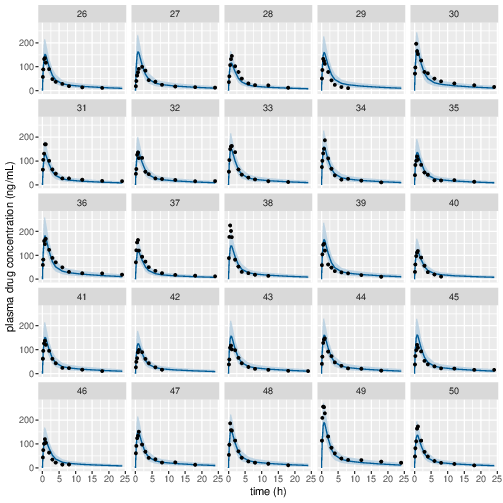
Figure 4: Predicted (90% credible interval and median) and observed individual plasma drug concentrations in study 1 (10mg dose).
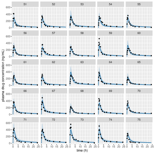
Figure 5: Predicted (90% credible interval and median) and observed individual plasma drug concentrations in study 1 (20mg dose).
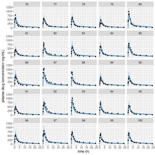
Figure 6: Predicted (90% credible interval and median) and observed individual plasma drug concentrations in study 1 (40mg dose).
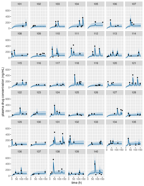
Figure 7: Predicted (90% credible interval and median) and observed individual plasma drug concentrations in study 2 (first 40 subjects).
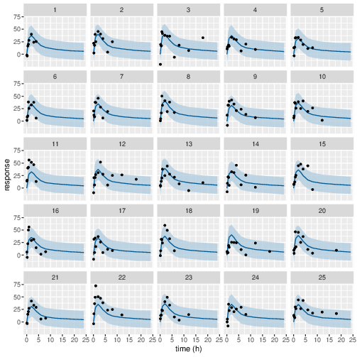
Figure 8: Predicted (90% credible interval and median) and observed individual PD response in study 1 (5mg dose).
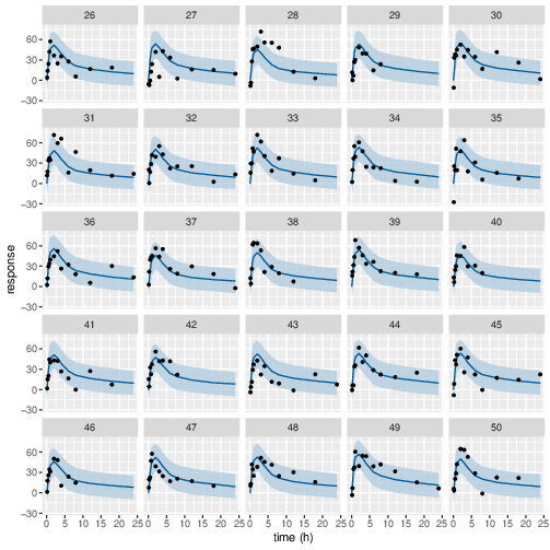
Figure 9: Predicted (90% credible interval and median) and observed individual PD response in study 1 (10mg dose).
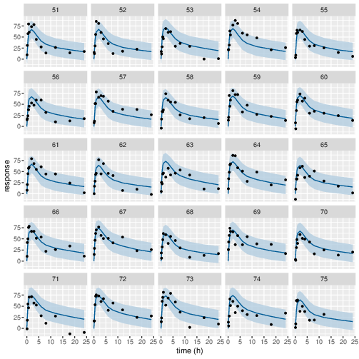
Figure 10: Predicted (90% credible interval and median) and observed individual PD response in study 1 (20mg dose).
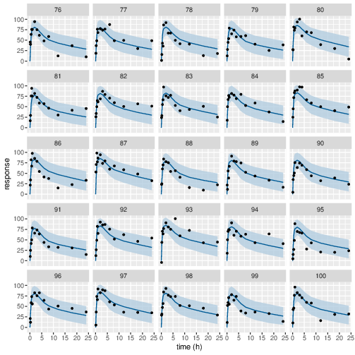
Figure 11: Predicted (90% credible interval and median) and observed individual PD response in study 1 (40mg dose).
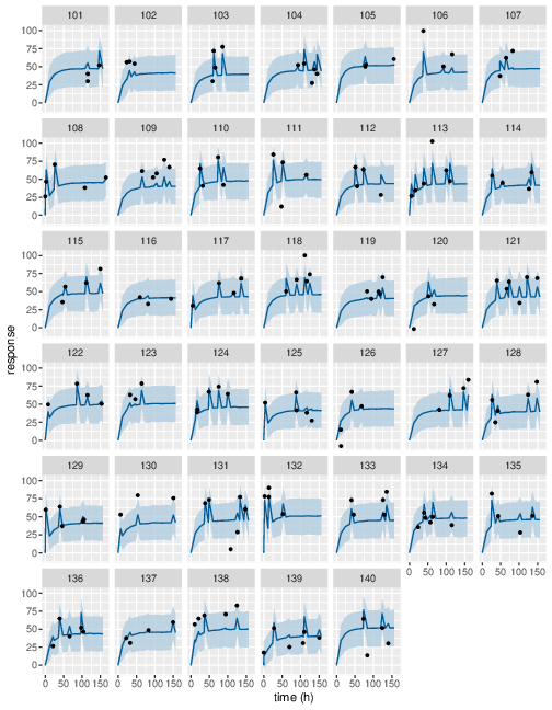
Figure 12: Predicted (90% credible interval and median) and observed individual PD response in study 2 (first 40 subjects).