Friberg-Karlsson Semi-Mechanistic Population Model
We now return to the example of Joint PK-PD model and extend it to a population model. While we recommend using the coupled solver, and this time we solve it using group solver. We leave it as an exercise to the reader to rewrite the model with coupled solver.
1 Friberg-Karlsson Population Model for drug-induced myelosuppression (\(ANC\))
\begin{gather*}
\log(ANC_{ij}) \sim N(Circ_{ij}, \sigma^2_{ANC}), \\\
\log\left(MTT_j, Circ_{0j}, \alpha_j\right) \sim N\left(\log\left(\widehat{MTT}, \widehat{Circ_0}, \widehat{\alpha}\right), \Omega_{ANC}\right), \\\
\left(\widehat{MTT}, \widehat{Circ}_0,\widehat{\alpha}, \gamma \right) = \left(125, 5, 2, 0.17\right), \\\
\Omega_{ANC} = \left(\begin{array}{ccc} 0.2^2 & 0 & 0 \ 0 & 0.35^2 & 0 \ 0 & 0 & 0.2^2 \end{array}\right), \\\
\sigma_{ANC} = 0.1, \\\
\Omega_{PK} = \left(\begin{array}{ccccc} 0.25^2 & 0 &a 0 & 0 & 0 \ 0 & 0.4^2 & 0 & 0 & 0 \\\
0 & 0 & 0.25^2 & 0 & 0 \ 0 & 0 & 0 & 0.4^2 & 0 \ 0 & 0 & 0 & 0 & 0.25^2 \end{array}\right)
\end{gather*}
The PK and the PD data are simulated using the following treatment.
- Phase IIa trial in patients
- Multiple doses: 80,000 mg
- Parallel dose escalation design
- 15 subjects
- PK: plasma concentration of parent drug (\(c\))
- PD response: Neutrophil count (\(ANC\))
- PK measured at 0.083, 0.167, 0.25, 0.5, 0.75, 1, 2, 3, 4, 6, 8, 12, 18, and 24 hours
- PD measured once every two days for 28 days.
Once again, we simultaneously fit the model to the PK and the PD data. It pays off to construct informative priors. For instance, we could fit the PK data first, as was done in example 1, and get informative priors on the PK parameters. The PD parameters are drug independent, so we can use information from the neutropenia literature. In this example, we choose to use strongly informative priors on both PK and PD parameters.
The ODE is defined as
functions{
    vector twoCptNeutModelODE(real t, vector x, real[] parms, real[] rdummy, int[] idummy){
    real k10;
    real k12;
    real k21;
    real CL;
    real Q;
    real V1;
    real V2;
    real ka;
    real mtt;
    real circ0;
    real gamma;
    real alpha;
    real ktr;
    vector[8] dxdt;
    real conc;
    real EDrug;
    real transit1;
    real transit2;
    real transit3;
    real circ;
    real prol;

    CL = parms[1];
    Q = parms[2];
    V1 = parms[3];
    V2 = parms[4];
    ka = parms[5];
    mtt = parms[6];
    circ0 = parms[7];
    gamma = parms[8];
    alpha = parms[9];

    k10 = CL / V1;
    k12 = Q / V1;
    k21 = Q / V2;

    ktr = 4 / mtt;

    dxdt[1] = -ka * x[1];
    dxdt[2] = ka * x[1] - (k10 + k12) * x[2] + k21 * x[3];
    dxdt[3] = k12 * x[2] - k21 * x[3];
    conc = x[2]/V1;
    EDrug = alpha * conc;
    // x[4], x[5], x[6], x[7] and x[8] are differences from circ0.
    prol = x[4] + circ0;
    transit1 = x[5] + circ0;
    transit2 = x[6] + circ0;
    transit3 = x[7] + circ0;
    circ = fmax(machine_precision(), x[8] + circ0); // Device for implementing a modeled
                                                    // initial condition
    dxdt[4] = ktr * prol * ((1 - EDrug) * ((circ0 / circ)^gamma) - 1);
    dxdt[5] = ktr * (prol - transit1);
    dxdt[6] = ktr * (transit1 - transit2);
    dxdt[7] = ktr * (transit2 - transit3);
    dxdt[8] = ktr * (transit3 - circ);

    return dxdt;
  }
}
We use the pmx_solve_group_rk45 function to
solve the entire population’s events.
transformed parameters{
  row_vector[nt] cHat;
  vector[nObsPK] cHatObs;
  row_vector[nt] neutHat;
  vector[nObsPD] neutHatObs;
  matrix[8, nt] x;
  real<lower = 0> parms[nSubjects, nTheta]; // The [1] indicates the parameters are constant

  // variables for Matt's trick
  vector<lower = 0>[nIIV] thetaHat;
  matrix<lower = 0>[nSubjects, nIIV] thetaM;

  // Matt's trick to use unit scale
  thetaHat[1] = CLHat;
  thetaHat[2] = QHat;
  thetaHat[3] = V1Hat;
  thetaHat[4] = V2Hat;
  thetaHat[5] = mttHat;
  thetaHat[6] = circ0Hat;
  thetaHat[7] = alphaHat;
  thetaM = (rep_matrix(thetaHat, nSubjects) .*
             exp(diag_pre_multiply(omega, L * etaStd)))';

  for(i in 1:nSubjects) {
    parms[i, 1] = thetaM[i, 1] * (weight[i] / 70)^0.75; // CL
    parms[i, 2] = thetaM[i, 2] * (weight[i] / 70)^0.75; // Q
    parms[i, 3] = thetaM[i, 3] * (weight[i] / 70); // V1
    parms[i, 4] = thetaM[i, 4] * (weight[i] / 70); // V2
    parms[i, 5] = kaHat; // ka
    parms[i, 6] = thetaM[i, 5]; // mtt
    parms[i, 7] = thetaM[i, 6]; // circ0
    parms[i, 8] = gamma;
    parms[i, 9] = thetaM[i, 7]; // alpha
  }

  /* group solver */
  x = pmx_solve_group_rk45(twoCptNeutModelODE, 8, len,
                           time, amt, rate, ii, evid, cmt, addl, ss,
                           parms,
                           1e-6, 1e-6, 500);

  for(i in 1:nSubjects) {
    cHat[start[i]:end[i]] = x[2, start[i]:end[i]] / parms[i, 3]; // divide by V1
    neutHat[start[i]:end[i]] = x[8, start[i]:end[i]] + parms[i, 7]; // Add baseline
  }

  for(i in 1:nObsPK) cHatObs[i] = cHat[iObsPK[i]];
  for(i in 1:nObsPD) neutHatObs[i] = neutHat[iObsPD[i]];
}
This allows us to use within-chain paralleleisation to reduce simulation time. When run from cmdstan, each MPI run generates one chain, and we use 4 MPI runs to generate 4 chains.
# chain 1
mpiexec -n nproc ./FribergKarlsson sample adapt delta=0.95 data file=fribergkarlsson.data.R init=fribergkarlsson.init.R random seed=8765 id=1 output file=output.1.csv
# chain 2
mpiexec -n nproc ./FribergKarlsson sample adapt delta=0.95 data file=fribergkarlsson.data.R init=fribergkarlsson.init.R random seed=8765 id=2 output file=output.2.csv
# chain 3
mpiexec -n nproc ./FribergKarlsson sample adapt delta=0.95 data file=fribergkarlsson.data.R init=fribergkarlsson.init.R random seed=8765 id=3 output file=output.3.csv
# chain 4
mpiexec -n nproc ./FribergKarlsson sample adapt delta=0.95 data file=fribergkarlsson.data.R init=fribergkarlsson.init.R random seed=8765 id=4 output file=output.4.csv
2 Results
Table FkpopModelParms summarizes the sampling and some diagnostics output. estimation reflects the real value of the parameters (Table FkpopModelParms and Figure fkpop_mcmc_density. Similar to the previous example, PPCs shown in Figure fkpop_ppc_pk and fkpop_ppc_pd indicate the model is a good fit.
| variable | mean | median | sd | mad | q5 | q95 | rhat | ess_bulk | ess_tail |
|---|---|---|---|---|---|---|---|---|---|
| CLHat | 9.539 | 9.535 | 0.522 | 0.487 | 8.692 | 10.401 | 1.006 | 971.369 | 1655.449 |
| QHat | 15.401 | 15.386 | 1.018 | 1.000 | 13.742 | 17.090 | 1.000 | 2263.843 | 2447.006 |
| V1Hat | 37.396 | 37.360 | 2.244 | 2.228 | 33.762 | 41.058 | 1.001 | 1936.476 | 2372.815 |
| V2Hat | 101.698 | 101.394 | 6.503 | 6.119 | 91.529 | 112.538 | 1.001 | 2580.227 | 2592.925 |
| kaHat | 1.997 | 1.997 | 0.074 | 0.074 | 1.873 | 2.115 | 1.001 | 7056.877 | 2993.406 |
| mttHat | 113.681 | 113.204 | 11.506 | 10.910 | 95.807 | 133.514 | 1.001 | 4255.900 | 3269.646 |
| circ0Hat | 4.760 | 4.752 | 0.241 | 0.229 | 4.375 | 5.163 | 1.002 | 3774.920 | 2783.663 |
| omega[1] | 0.223 | 0.217 | 0.047 | 0.042 | 0.160 | 0.307 | 1.000 | 1751.864 | 2235.607 |
| omega[2] | 0.339 | 0.329 | 0.073 | 0.067 | 0.239 | 0.473 | 1.001 | 2363.843 | 2607.056 |
| omega[3] | 0.264 | 0.256 | 0.057 | 0.051 | 0.186 | 0.367 | 1.002 | 2128.660 | 2018.425 |
| omega[4] | 0.257 | 0.249 | 0.056 | 0.051 | 0.182 | 0.361 | 1.003 | 2293.877 | 2937.673 |
| omega[5] | 0.177 | 0.169 | 0.112 | 0.118 | 0.019 | 0.376 | 1.000 | 1550.483 | 2045.025 |
| omega[6] | 0.188 | 0.183 | 0.044 | 0.041 | 0.127 | 0.269 | 1.000 | 2377.698 | 2965.713 |
| omega[7] | 0.409 | 0.394 | 0.256 | 0.259 | 0.045 | 0.865 | 1.003 | 1386.987 | 2015.873 |
| gamma | 0.171 | 0.168 | 0.035 | 0.033 | 0.121 | 0.235 | 1.000 | 8809.668 | 3189.676 |
| sigma | 0.097 | 0.096 | 0.003 | 0.003 | 0.093 | 0.101 | 1.002 | 5436.508 | 2899.706 |
| sigmaNeut | 0.106 | 0.105 | 0.012 | 0.011 | 0.088 | 0.127 | 1.000 | 2809.059 | 3031.605 |
| alphaHat | 2.24e-4 | 2.19e-4 | 3.97e-05 | 3.80e-05 | 1.66e-4 | 2.96e-4 | 1.000 | 5138.105 | 2807.328 |
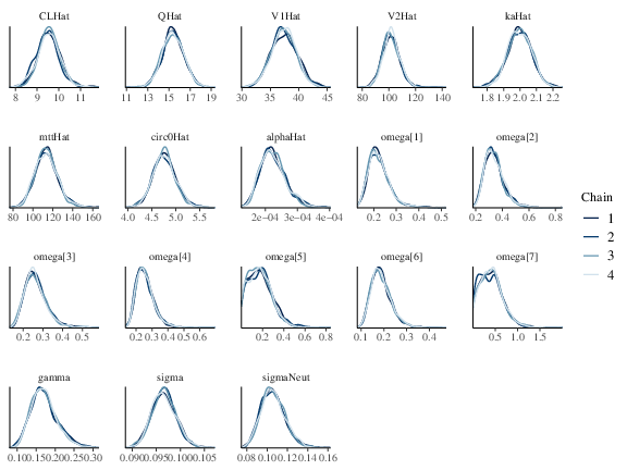
Figure 1: Posterior marginal densities of the model parameters of the Friberg-Karlsson population model.
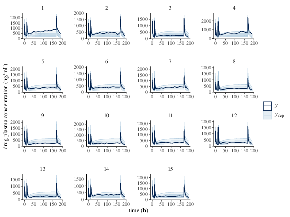
Figure 2: Predicted (50%, 90% credible interval and median) and observed individual drug plasma concentration.
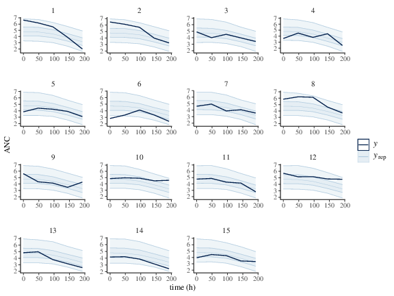
Figure 3: Predicted (50%, 90% credible interval and median) and observed individual Neutrophil counts.
\appendix