Joint PK-PD model
Neutropenia is observed in patients receiving an ME-2 drug. Our goal is to model the relation between neutrophil counts and drug exposure. As shown in Figure 1, the Friberg-Karlsson Semi-Mechanistic model (Friberg and Karlsson 2003) couples a PK model with a PD effect to describe a delayed feedback mechanism that keeps the absolute neutrophil count (ANC) at the baseline in a circulatory compartment (Circ), and the drug’s effect in reducing the proliferation rate (prol). The delay between prol and Circ is modeled using \(n\) transit comparments with mean transit time MTT = \((n + 1)/k_{\text{tr}}\), with \(k_{\text{tr}}\) the transit rate constant. In the current example, we use the Two Compartment Model for PK model, and set \(n = 3\).
\begin{align}
\log(\text{ANC})& \sim N(\log(y_{\text{circ}}), \sigma^2_{\text{ANC}}), \\\
y_{\text{circ}}& = f_{\text{FK}}(\text{MTT}, \text{Circ}_{0}, \alpha, \gamma, c),
\end{align}
where \(c\) is the drug concentration calculated from the PK model, and function \(f_{\text{FK}}\) represents solving the following nonlinear ODE for \(y_{\text{circ}}\)
\begin{align}\label{eq:FK}
\frac{dy_\mathrm{prol}}{dt} &= k_\mathrm{prol} y_\mathrm{prol} (1 - E_\mathrm{drug})\left(\frac{\text{Circ}_0}{y_\mathrm{circ}}\right)^\gamma - k_\mathrm{tr}y_\mathrm{prol}, \\\
\frac{dy_\mathrm{trans1}}{dt} &= k_\mathrm{tr} y_\mathrm{prol} - k_\mathrm{tr} y_\mathrm{trans1}, \\\
\frac{dy_\mathrm{trans2}}{dt} &= k_\mathrm{tr} y_\mathrm{trans1} - k_\mathrm{tr} y_\mathrm{trans2}, \\\
\frac{dy_\mathrm{trans3}}{dt} &= k_\mathrm{tr} y_\mathrm{trans2} - k_\mathrm{tr} y_\mathrm{trans3}, \\\
\frac{dy_\mathrm{circ}}{dt} &= k_\mathrm{tr} y_\mathrm{trans3} - k_\mathrm{tr} y_\mathrm{circ},
\end{align}
We use \(E_{\text{drug}} = \alpha c\) to model the linear effect of drug concentration in central compartment, with \(c=y_{\text{cent}}/V_{\text{cent}}\) based on PK solutions.
Since the ODEs specifying the Two Compartment Model
(Equation \eqref{eq:twocpt}) do not depend on the PD ODEs
(Equation \eqref{eq:FK}) and can be solved analytically
using Torsten’s pmx_solve_twocpt function
we can specify solve the system using a coupled solver function. We do not
expect our system to be stiff and use the Runge-Kutta 4th/5th order
integrator.
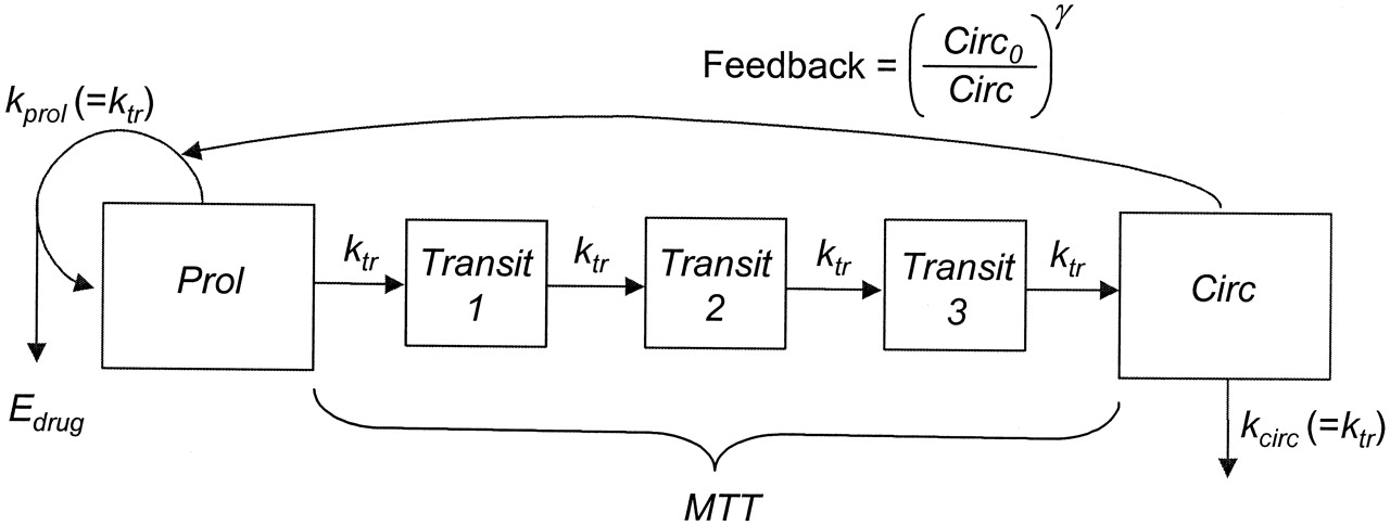
Figure 1: Friberg-Karlsson semi-mechanistic Model.
The model fitting is based on simulated data
\begin{align*}
(\text{MTT}, \text{Circ}_{0}, \alpha, \gamma, k_{\text{tr}})& = (125, 5.0, 3 \times 10^{-4}, 0.17) \\\
\sigma^2_{\text{ANC}}& = 0.001.
\end{align*}
functions{
  vector FK_ODE(real t, vector y, vector y_pk, real[] theta, real[] rdummy, int[] idummy){
    /* PK variables */
    real VC = theta[3];

    /* PD variable */
    real mtt      = theta[6];
    real circ0    = theta[7];
    real alpha    = theta[8];
    real gamma    = theta[9];
    real ktr      = 4.0 / mtt;
    real prol     = y[1] + circ0;
    real transit1 = y[2] + circ0;
    real transit2 = y[3] + circ0;
    real transit3 = y[4] + circ0;
    real circ     = fmax(machine_precision(), y[5] + circ0);
    real conc     = y_pk[2] / VC;
    real EDrug    = alpha * conc;

    vector[5] dydt;

    dydt[1] = ktr * prol * ((1 - EDrug) * ((circ0 / circ)^gamma) - 1);
    dydt[2] = ktr * (prol - transit1);
    dydt[3] = ktr * (transit1 - transit2);
    dydt[4] = ktr * (transit2 - transit3);
    dydt[5] = ktr * (transit3 - circ);

    return dydt;
  }
}

data{
  int<lower = 1> nt;
  int<lower = 1> nObsPK;
  int<lower = 1> nObsPD;
  int<lower = 1> iObsPK[nObsPK];
  int<lower = 1> iObsPD[nObsPD];
  real<lower = 0> amt[nt];
  int<lower = 1> cmt[nt];
  int<lower = 0> evid[nt];
  real<lower = 0> time[nt];
  real<lower = 0> ii[nt];
  int<lower = 0> addl[nt];
  int<lower = 0> ss[nt];
  real rate[nt];
  vector<lower = 0>[nObsPK] cObs;
  vector<lower = 0>[nObsPD] neutObs;

  real<lower = 0> circ0Prior;
  real<lower = 0> circ0PriorCV;
  real<lower = 0> mttPrior;
  real<lower = 0> mttPriorCV;
  real<lower = 0> gammaPrior;
  real<lower = 0> gammaPriorCV;
  real<lower = 0> alphaPrior;
  real<lower = 0> alphaPriorCV;
}

transformed data{
  int nOde = 5;
  vector[nObsPK] logCObs;
  vector[nObsPD] logNeutObs;

  int nTheta = 9; // number of parameters
  int nIIV = 7; // parameters with IIV

  int n = 8;                        /* ODE dimension */
  real rtol = 1e-8;
  real atol = 1e-8;;
  int max_step = 100000;

  logCObs = log(cObs);
  logNeutObs = log(neutObs);
}

parameters{

  real<lower = 0> CL;
  real<lower = 0> Q;
  real<lower = 0> VC;
  real<lower = 0> VP;
  real<lower = 0> ka;
  real<lower = 0> mtt;
  real<lower = 0> circ0;
  real<lower = 0> alpha;
  real<lower = 0> gamma;
  real<lower = 0> sigma;
  real<lower = 0> sigmaNeut;

  // IIV parameters
  cholesky_factor_corr[nIIV] L;
  vector<lower = 0>[nIIV] omega;
}

transformed parameters{
  row_vector[nt] cHat;
  vector<lower = 0>[nObsPK] cHatObs;
  row_vector[nt] neutHat;
  vector<lower = 0>[nObsPD] neutHatObs;
  real<lower = 0> theta[nTheta];
  matrix[nOde + 3, nt] x;
  real biovar[nTheta] = rep_array(1.0, nTheta);
  real tlag[nTheta] = rep_array(0.0, nTheta);

  theta[1] = CL;
  theta[2] = Q;
  theta[3] = VC;
  theta[4] = VP;
  theta[5] = ka;
  theta[6] = mtt;
  theta[7] = circ0;
  theta[8] = alpha;
  theta[9] = gamma;

  x = pmx_solve_twocpt_rk45(FK_ODE, nOde, time, amt, rate, ii, evid, cmt, addl, ss, theta, biovar, tlag, rtol, atol, max_step);

  cHat = x[2, ] / VC;
  neutHat = x[8, ] + circ0;

  for(i in 1:nObsPK) cHatObs[i]    = cHat[iObsPK[i]];
  for(i in 1:nObsPD) neutHatObs[i] = neutHat[iObsPD[i]];
}

model {
  // Priors
  CL    ~ normal(0, 20);
  Q     ~ normal(0, 20);
  VC    ~ normal(0, 100);
  VP    ~ normal(0, 1000);
  ka    ~ normal(0, 5);
  sigma ~ cauchy(0, 1);

  mtt       ~ lognormal(log(mttPrior), mttPriorCV);
  circ0     ~ lognormal(log(circ0Prior), circ0PriorCV);
  alpha     ~ lognormal(log(alphaPrior), alphaPriorCV);
  gamma     ~ lognormal(log(gammaPrior), gammaPriorCV);
  sigmaNeut ~ cauchy(0, 1);

  // Parameters for Matt's trick
  L ~ lkj_corr_cholesky(1);
  omega ~ cauchy(0, 1);

  // observed data likelihood
  logCObs ~ normal(log(cObs), sigma);
  logNeutObs ~ normal(log(neutObs), sigmaNeut);
}
1 Bibliography
Friberg, Lena E., and Mats O. Karlsson. 2003. “Mechanistic Models for Myelosuppression.” Investigational New Drugs 21 (2):183–94. https://link.springer.com/article/10.1023/A:1023573429626.