Two-compartment model for single patient
We model drug absorption in a single patient and simulate plasma drug concentrations:
- Multiple Doses: 1250 mg, every 12 hours, for a total of 15 doses
- PK measured at 0.083, 0.167, 0.25, 0.5, 0.75, 1, 1.5, 2, 4, 6, 8, 10 and 12 hours after 1st, 2nd, and 15th dose. In addition, the PK is measured every 12 hours throughout the trial.
With the plasma concentration \(\hat{c}\) using Two Compartment Model, we simulate \(c\) according to:
\begin{align*}
\log\left(c\right) &\sim N\left(\log\left(\widehat{c}\right),\sigma^2\right) \\\
\left(CL, Q, V_2, V_3, ka\right) &= \left(5\ {\rm L/h}, 8\ {\rm L/h}, 20\ {\rm L}, 70\ {\rm L}, 1.2\ {\rm h^{-1}} \right) \\\
\sigma^2 &= 0.01
\end{align*}
The data are generated using the R package mrgsolve (Baron and Gastonguay 2015).
Code below shows how Torsten function pmx_solve_twocpt can be used to fit the above model.
data{
  int<lower = 1> nt;  // number of events
  int<lower = 1> nObs;  // number of observation
  int<lower = 1> iObs[nObs];  // index of observation

  // NONMEM data
  int<lower = 1> cmt[nt];
  int evid[nt];
  int addl[nt];
  int ss[nt];
  real amt[nt];
  real time[nt];
  real rate[nt];
  real ii[nt];

  vector<lower = 0>[nObs] cObs;  // observed concentration (Dependent Variable)
}

transformed data{
  vector[nObs] logCObs = log(cObs);
  int nTheta = 5;  // number of ODE parameters in Two Compartment Model
  int nCmt = 3;  // number of compartments in model
}

parameters{
  real<lower = 0> CL;
  real<lower = 0> Q;
  real<lower = 0> V1;
  real<lower = 0> V2;
  real<lower = 0> ka;
  real<lower = 0> sigma;
}

transformed parameters{
  real theta[nTheta];  // ODE parameters
  row_vector<lower = 0>[nt] cHat;
  vector<lower = 0>[nObs] cHatObs;
  matrix<lower = 0>[nCmt, nt] x;

  theta[1] = CL;
  theta[2] = Q;
  theta[3] = V1;
  theta[4] = V2;
  theta[5] = ka;

  x = pmx_solve_twocpt(time, amt, rate, ii, evid, cmt, addl, ss, theta);

  cHat = x[2, :] ./ V1; // we're interested in the amount in the second compartment

  cHatObs = cHat'[iObs]; // predictions for observed data recors
}

model{
  // informative prior
  CL ~ lognormal(log(10), 0.25);
  Q ~ lognormal(log(15), 0.5);
  V1 ~ lognormal(log(35), 0.25);
  V2 ~ lognormal(log(105), 0.5);
  ka ~ lognormal(log(2.5), 1);
  sigma ~ cauchy(0, 1);

  logCObs ~ normal(log(cHatObs), sigma);
}
Four MCMC chains of 2000 iterations (1000 warmup iterations and 1000
sampling iterations) are simulated. 1000 samples per chain were used for the subsequent analyses.
The MCMC history plots(Figure 1)
suggest that the 4 chains have converged to common distributions for
all of the key model parameters. The fit to the plasma concentration
data (Figure 3) are in close agreement with the
data, which is not surprising since the fitted model is identical to
the one used to simulate the data. Similarly the parameter posterior
density can be examined in Figure 2 and shows
consistency with the values used for simulation. Another way to
summarize the posterior is through cmdstanr’s summary method.
## fit is a CmdStanMCMC object returned by sampling. See cmdstanr reference.
> pars = c("CL", "Q", "V1", "V2", "ka", "sigma")
> fit$summary(pars)
# A tibble: 6 x 10
  variable   mean median     sd    mad      q5    q95  rhat ess_bulk ess_tail
  <chr>     <dbl>  <dbl>  <dbl>  <dbl>   <dbl>  <dbl> <dbl>    <dbl>    <dbl>
1 CL        4.82   4.83  0.0910 0.0870  4.68    4.97   1.00    1439.    1067.
2 Q         7.56   7.55  0.588  0.586   6.61    8.56   1.00    1256.    1235.
3 V1       21.1   21.1   2.50   2.45   17.1    25.3    1.00    1057.    1177.
4 V2       76.1   76.1   5.33   4.93   67.5    84.9    1.01    1585.    1372.
5 ka        1.23   1.23  0.175  0.174   0.958   1.52   1.00    1070.    1122.
6 sigma     0.109  0.108 0.0117 0.0111  0.0911  0.130  1.01    1414.     905.
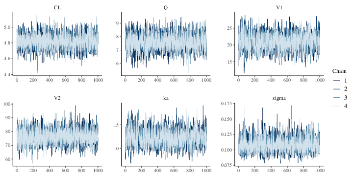
Figure 1: MCMC history plots for the parameters of a two compartment model with first order absorption (each color corresponds to a different chain)
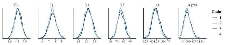
Figure 2: Posterior marginal densities of the Model Parameters of a two compartment model with first order absorption (each color corresponds to a different chain)
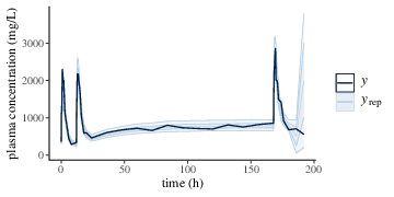
Figure 3: Predicted (\(y_{\text{rep}}\)) and observed (\(y\)) plasma drug concentrations of a two compartment model with first order absorption. \(y_{\text{rep}}\) is shown with posterior median, 50%, 90% credible intervals.
Bibliography
Baron, Kyle T., and Marc R. Gastonguay. 2015. “Simulation from ODE-Based Population PK/PD and Systems Pharmacology Models in R with Mrgsolve.” Journal of Pharmacokinetics and Pharmacodynamics 42 (W-23):S84–85.