pmplots is a package for R to make simple, standardized plots in a pharmacometric data analysis environment. The goal with this package isn’t to create a new grammar of graphics, but rather to create a standard set of commonly-used plots in pharmacometrics analyses.
This quick start chapter is meant to give you a brief orientation about how pmplots works. A more complete treatment is given in subsequent chapters.
2.1 Basic idea
The most basic functionality provided by pmplots is a set of functions which accept data frame with standardized names and returns a single plot.
We will load some example data from the package to illustrate. This is a data set that is similar to what we usually have after a NONMEM estimation run
data <- pmplots::pmplots_data_obs()head(as.data.frame(data), n =3)
   C NUM ID SUBJ TIME SEQ CMT EVID AMT      DV   AGE    WT   CRCL ALB   BMI
1 NA   2  1    1 0.61   1   2    0  NA  61.005 28.03 55.16 114.45 4.4 21.67
2 NA   3  1    1 1.15   1   2    0  NA  90.976 28.03 55.16 114.45 4.4 21.67
3 NA   4  1    1 1.73   1   2    0  NA 122.210 28.03 55.16 114.45 4.4 21.67
     AAG  SCR   AST   ALT     HT CP TAFD  TAD LDOS MDV BLQ PHASE STUDY   RF 102
1 106.36 1.14 11.88 12.66 159.55  0 0.61 0.61    5   0   0     1     1 norm   1
2 106.36 1.14 11.88 12.66 159.55  0 1.15 1.15    5   0   0     1     1 norm   1
3 106.36 1.14 11.88 12.66 159.55  0 1.73 1.73    5   0   0     1     1 norm   1
   IPRED    CWRESI     NPDE   PRED      RES     WRES     CL     V2    KA
1 69.502 -0.621370 -0.62293 60.886  0.11865 -0.56749 2.5927 40.287 1.452
2 91.230  0.089509  0.27064 78.945 12.03100  0.13248 2.5927 40.287 1.452
3 97.076  1.598600  1.55480 83.523 38.68700  1.62720 2.5927 40.287 1.452
     ETA1     ETA2      ETA3 DOSE STUDYc    CPc     CWRES
1 -0.0753 -0.18403 -0.095308    5    SAD normal -0.621370
2 -0.0753 -0.18403 -0.095308    5    SAD normal  0.089509
3 -0.0753 -0.18403 -0.095308    5    SAD normal  1.598600
Another data set is based on data in the previous code chunk, but subset to just one record per individual
id <- pmplots::pmplots_data_id()
Some of the “standard” column names include
ID
TIME
NPDE
PRED
ETA1
We frequently see these names in NONMEM output and pmplots is set up to take advantage of this.
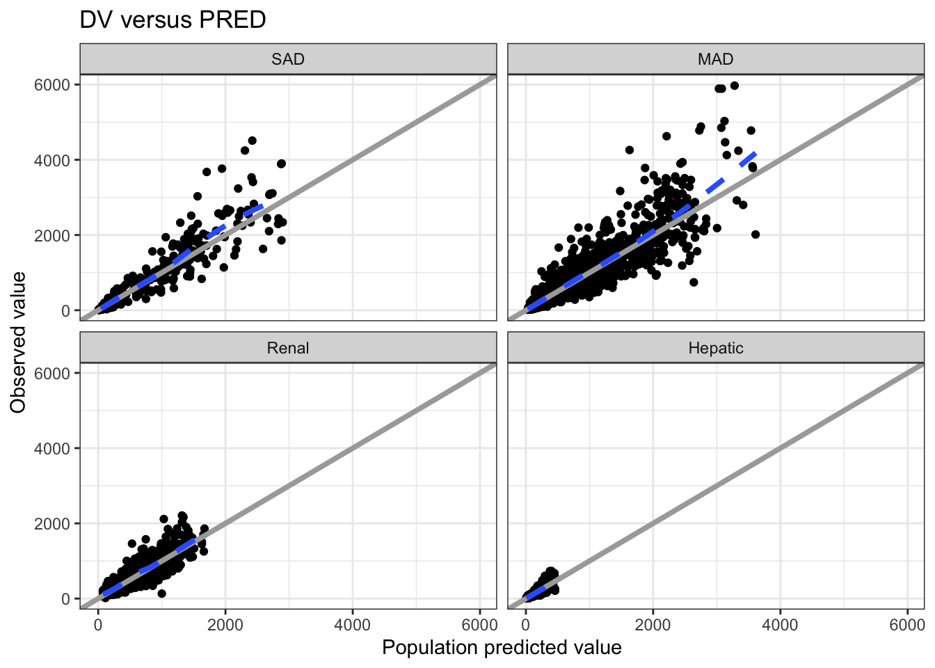
So to create a plot of DV (observed data points) versus PRED (population predictions) we call dv_pred()
dv_pred(data)
This default plot has the following features
The x- and y-axes are forced to have the same limits
There is reference line at x = y
There is a loess smooth through the data points
The idea is to create a simple, standardized plot with only minimal code. Of course, there are ways to customize this plot
These functions return gg objects so you can also continue to customize the plot as you normally would with ggplot2
dv_pred(data) +facet_wrap(~STUDYc) +ggtitle("DV versus PRED")
Other plots including DV, PRED and IPRED include
dv_time() (DV vs TIME)
dv_ipred() (DV vs IPRED)
dv_preds() (DV vs both PRED and IPRED)
3 Diagnostic plots
pmplots generates a host of residual diagnostics and similar plots (e.g. NPDE)
Conditional weighted residuals versus time
p1 <-cwres_time(data)
Residuals versus population predicted value
p2 <-res_pred(data)
NPDE boxplots in each study
p3 <-npde_cat(data, x ="STUDYc//Study")
Histogram of weighted residuals
p4 <-wres_hist(data)
With output
(p1+p2)/(p3+p4)
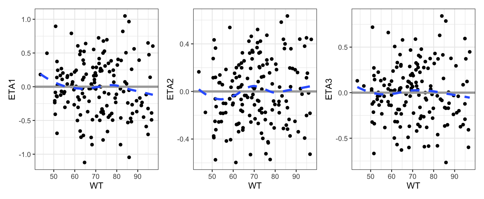
Diagnostic plots can be vectorized, getting returned in a list. Pass the list to pm_grid() to arrange them
eta_cont(id, x ="WT", y =paste0("ETA", c(1,2,3))) %>%pm_grid(ncol =3)
4 Exploratory plots
pmplots also makes plots for exploratory graphics.
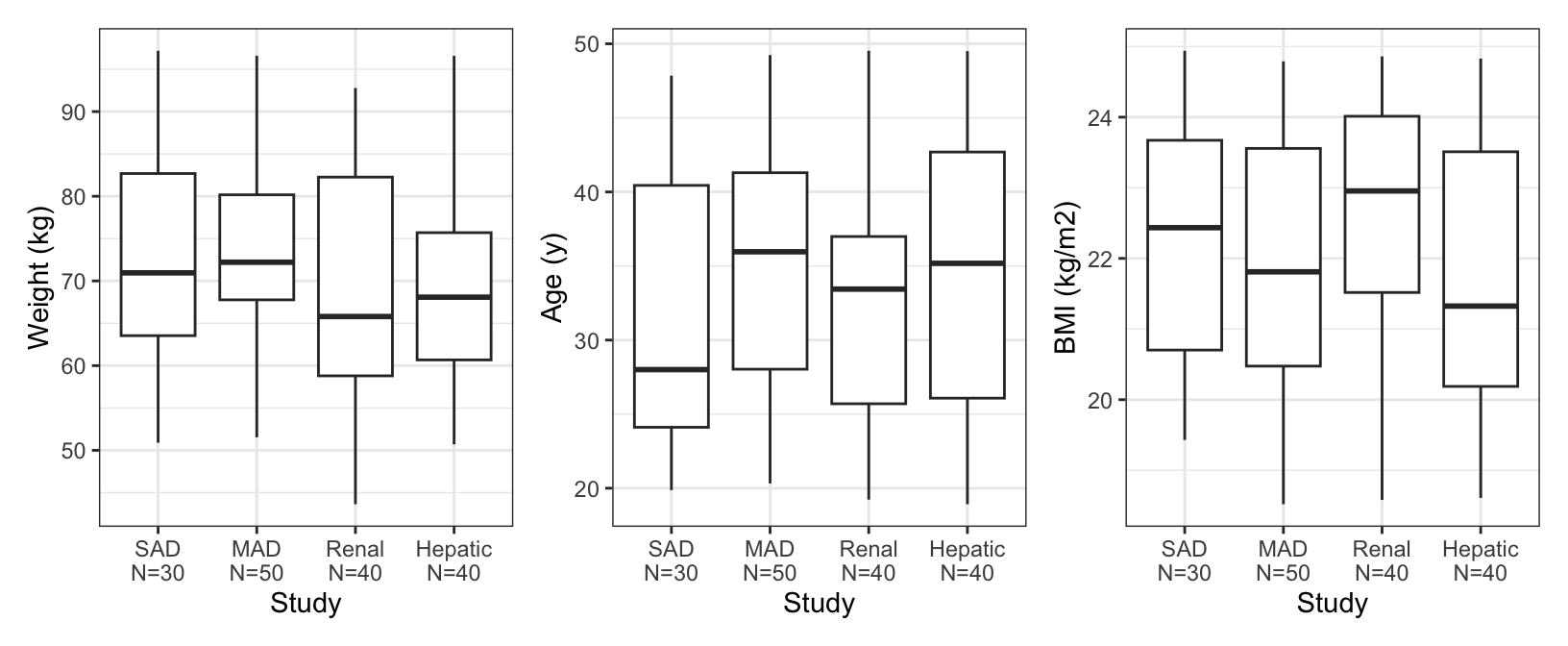
We can look at continuous covariates by another categorical covariate
covar <-c("WT//Weight (kg)", "AGE//Age (y)", "BMI//BMI (kg/m2)", "ALB//Albumin (g/dL)") cont_cat( id, x ="STUDYc//Study ", y = covar[1:3],) %>%pm_grid(ncol =3)
Or correlations between continuous covariates
pairs_plot(data, y = covar)
5 col-label
You might have noticed a special syntax that we’ve used in some of the previous plots. For example
npde_cat(data, x ="STUDYc//Study")
Here we are using col-label syntax. This is just a compact way to pass both the name of the column to plot and a more formal axis title. col-label are delimited (by default) by //
col_label("STUDYc//Study")
[1] "STUDYc" "Study"
After parsing, the left hand side is column name and the right hand side is the axis title.
It’s ok to just pass the left hand side too
col_label("STUDYc")
[1] "STUDYc" "STUDYc"
Here the axis title is just the column name.
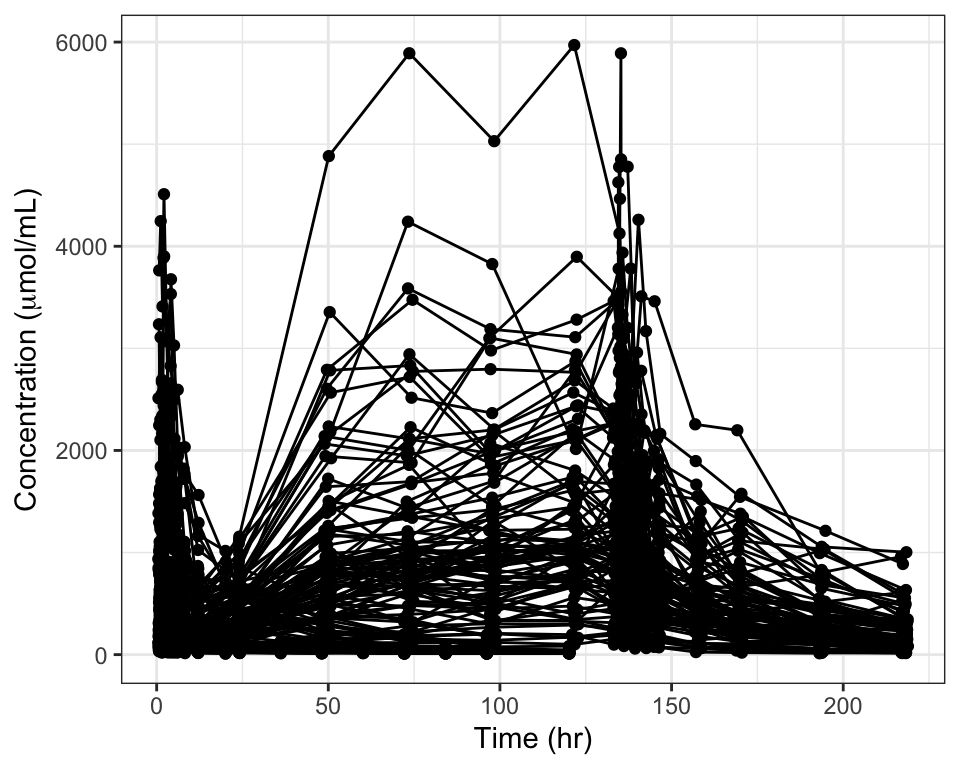
Axis titles can also contain a subset of TeX syntax that gets parsed by the latex2exp package
col_label("DV//$\\mu$mol/mL")
[1] "DV" "$\\mu$mol/mL"
For example
dv_time(data, y ="DV//Concentration ($\\mu$mol/mL)")