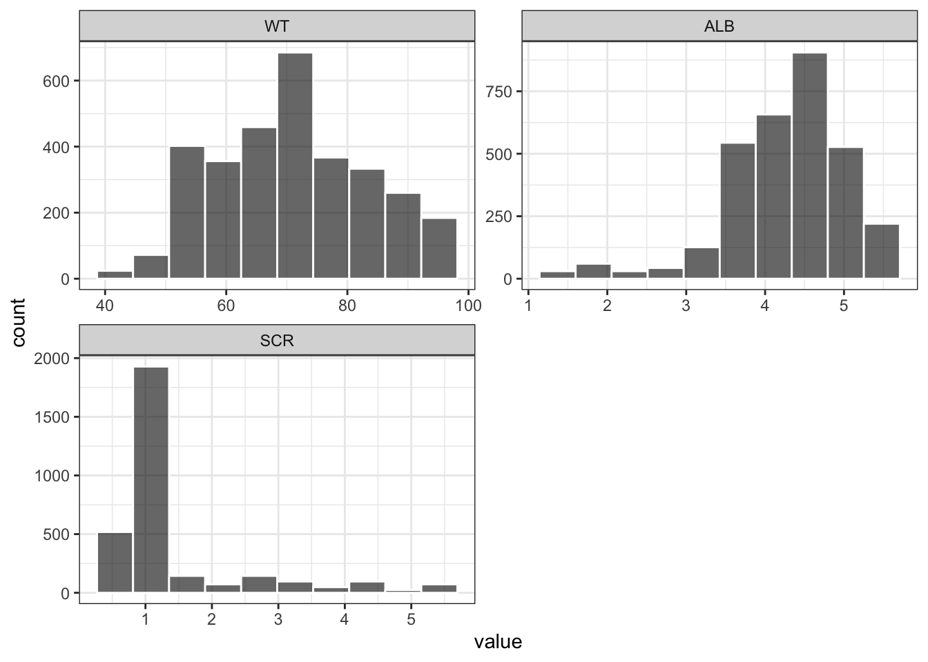
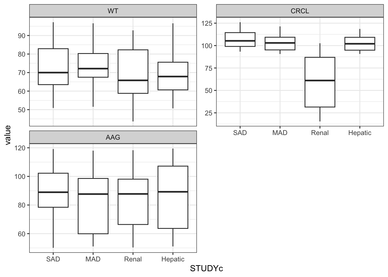
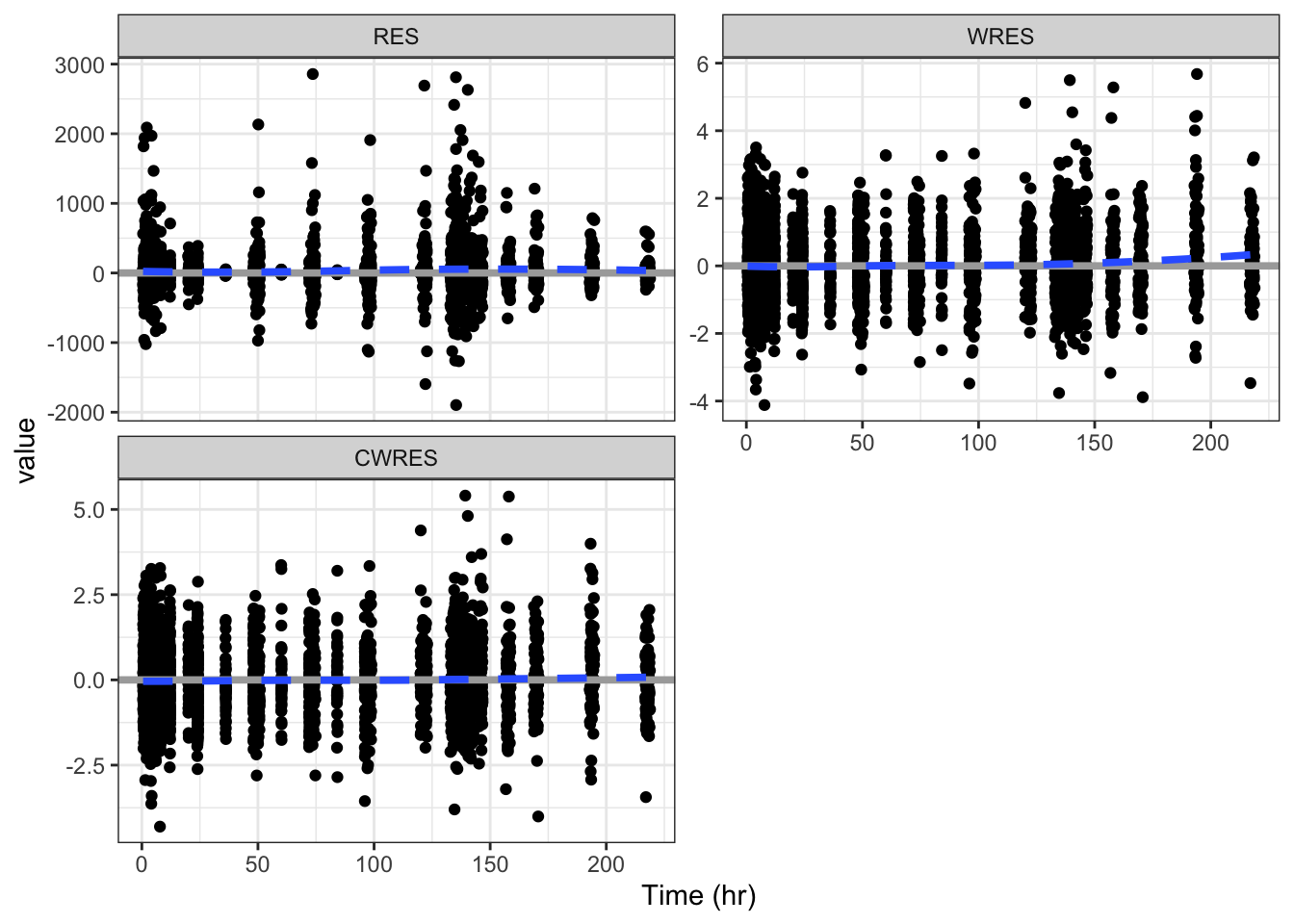
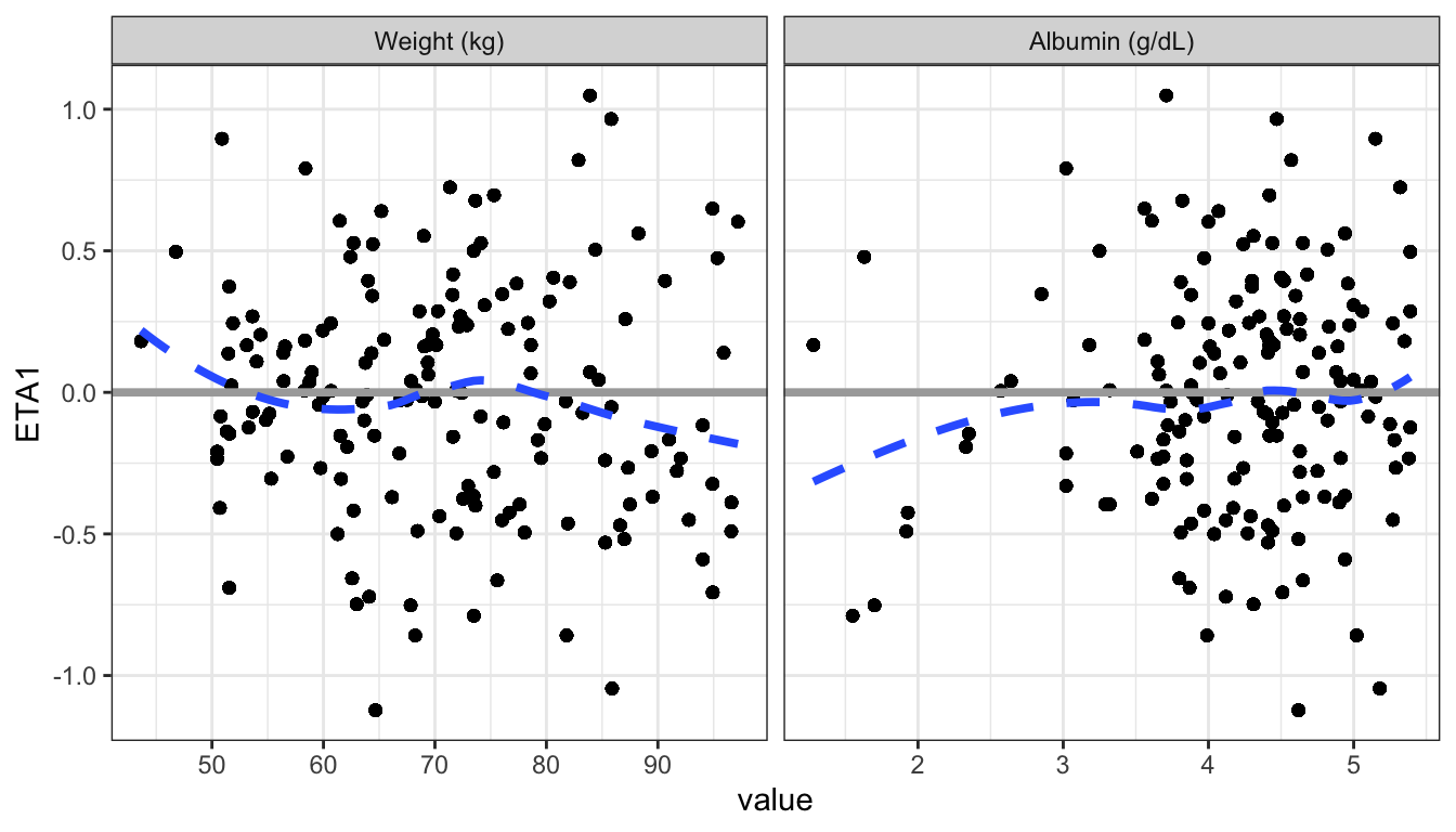
Wrapped plots are like the other standardized plots we have seen in the gallery so far, but they allow for a simple faceting using ggplot2::facet_wrap().
Preview the data used on this page
The data are identical to the data used for the other series of plots and do not require any special configuration.
head(as.data.frame(df), n=3)
   C NUM ID SUBJ TIME SEQ CMT EVID AMT      DV   AGE    WT   CRCL ALB   BMI
1 NA   2  1    1 0.61   1   2    0  NA  61.005 28.03 55.16 114.45 4.4 21.67
2 NA   3  1    1 1.15   1   2    0  NA  90.976 28.03 55.16 114.45 4.4 21.67
3 NA   4  1    1 1.73   1   2    0  NA 122.210 28.03 55.16 114.45 4.4 21.67
     AAG  SCR   AST   ALT     HT CP TAFD  TAD LDOS MDV BLQ PHASE STUDY   RF 102
1 106.36 1.14 11.88 12.66 159.55  0 0.61 0.61    5   0   0     1     1 norm   1
2 106.36 1.14 11.88 12.66 159.55  0 1.15 1.15    5   0   0     1     1 norm   1
3 106.36 1.14 11.88 12.66 159.55  0 1.73 1.73    5   0   0     1     1 norm   1
   IPRED    CWRESI     NPDE   PRED      RES     WRES     CL     V2    KA
1 69.502 -0.621370 -0.62293 60.886  0.11865 -0.56749 2.5927 40.287 1.452
2 91.230  0.089509  0.27064 78.945 12.03100  0.13248 2.5927 40.287 1.452
3 97.076  1.598600  1.55480 83.523 38.68700  1.62720 2.5927 40.287 1.452
     ETA1     ETA2      ETA3 DOSE STUDYc    CPc     CWRES
1 -0.0753 -0.18403 -0.095308    5    SAD normal -0.621370
2 -0.0753 -0.18403 -0.095308    5    SAD normal  0.089509
3 -0.0753 -0.18403 -0.095308    5    SAD normal  1.598600